


As energy production from offshore wind expands, new and deeper ocean areas are being considered for development. As discussed in Chapter 4, floating support structures should be considered for water depths beyond 50 m. Floating support structures introduce several new aspects with respect to dynamic behavior compared to bottom-fixed support structures. These aspects will be discussed in more detail in this chapter.
The starting point is equations of motion for a rigid body in six degrees of freedom (6DOF). The forcing mechanisms from waves are addressed as well as the inertia effects due to the surrounding fluid, the added mass, hydrostatics and the effect of mooring. The effect of wind forces is discussed in Chapter 3. This chapter further discusses the combined effect of wind forces and the motion control system.
Floating support structures can take several geometric shapes. Various methods for computing the wave loads on rectangular pontoons, barges etc. will therefore be outlined in more detail. In Chapter 6, the boundary element method for computing wave loads on a 3D body of general shape was discussed. This method is well suited also for floating bodies. However, simpler and computationally faster methods are useful in the design process, in particular for optimization purposes. Therefore, strip theory methods are outlined in some detail. Most of the derivations in this chapter are based upon linear methods. This implies that forces are computed at the initial or mean position of the structure, and that inertia, damping and restoring effects are also linearized and referred to the initial or mean position. The linearization also implies that all dynamic rotations of the support structure are assumed to be small. The linearization makes the computations efficient and allows for solving the dynamics in the frequency domain. However, in real design processes the importance of various nonlinear effects must be assessed.
For floating support structures, a great variety of shapes have been proposed, as illustrated in Chapter 4. In most cases the floater is assembled of slender horizontal pontoons and vertical columns. Both the pontoons and the columns may have a cross-sectional area that varies along the length. In addition, flat solid or perforated plates may be introduced to obtain the wanted dynamic characteristics of the floater. Some floating foundations have a barge-like shape; thus, the applicability and accuracy of the various methods must be evaluated for each case. For example, in a preliminary design phase involving an optimization process, strip theory methods may be applied. Having concluded on a geometry, the results obtained by strip theory should be compared to results obtained by 3D methods.
7.1 Wave-Induced Motions: Equations of Motion
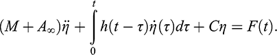
Considering the six rigid-body degrees of motion, the dynamic equations may be written as:
 ([7.1])
Here,
 is the vector of the six degrees of motion, as illustrated in Figure 7.1. The figure also shows the common naming convention for the motions. The linear motions in direction
 are denoted
 and the rotations about the
 axes are denoted
 . It is here is assumed that the
 -plane coincides with the mean water surface and that
 is vertical, zero at the mean free surface and positive upward.
 is the 6 x 6 dry mass matrix of the complete wind turbine and
 is the hydrodynamic mass matrix. The damping matrix is split into two parts, the radiation part,
 , related to wave generation, and the remaining damping,
 , mainly linearized viscous damping from water and air. The damping could also contain effects due to the control of the wind turbine, but these effects may also be included in the forcing term. The restoring matrix is split into a hydrostatic part,
 , and a mooring part,
 . The four excitation force vectors are the wave force vector; the wind force on the structural parts; the current force; and the force due to the action of the wind turbine.

If the equations are linearized, [7.1], and a stationary, dynamic response is considered, the force vector may be written as
 and the response as
 , where
 is the frequency of oscillation and
 is the complex response vector. The equation of motion in frequency domain may thus be written as:
 ([7.2])
Here, it is indicated that in the general case, the added mass as well as the damping are frequency-dependent. The frequency domain format of the equation of motions is useful when wave forces dominate the excitation. If significant nonlinear effects are present, which is the case for wind turbines during operation and active control functions, the equations must be written and solved in time domain. If the hydrodynamic forces are assumed to be linear but frequency-dependent, a convolution integral is needed in the time domain version of the equations to account for the frequency dependence. In time domain the frequency dependence represents a memory effect. In the 1D case the equation of motion in time domain may then be written as:
 ([7.3])
The convolution term now accounts for the frequency dependency of added mass and damping (these are related) and
 is the high-frequency limit of the added mass. Further discussion of time domain formulation of the equation of motion with frequency-dependent coefficients is found in, e.g., Reference FalnesFalnes (2002). Further details are given in Section 7.4.8.
7.2 The Mass Matrix
7.2.1 The Dry Mass Matrix
The mass matrix for the dry body can be written as:
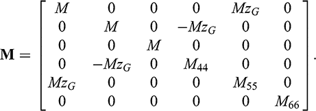 ([7.4])
Here, it assumed that the center of gravity (CG) is located at
 and that the
 and the
 -planes are planes of symmetry, which frequently is the case for floating bodies.
 is the mass of the body, and the moments of inertia are given by:
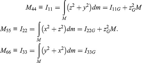 ([7.5])
Here,
 refers to the mass moment of inertia about axis
 and
and
 refers to the mass moment when the axis has origin in CG.
In the more general case without symmetry and where the CG is located in
 , the mass matrix may be obtained by:
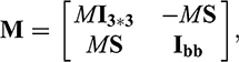 ([7.6])
where

For further details, see Reference Perez and FossenPerez and Fossen (2007).
7.2.2 The Added Mass Matrix
In many of the proposed designs for offshore wind support structures, the floater is composed of slender horizontal pontoons and vertical columns. Both the pontoons and the columns may have a cross-sectional area that varies along its length. In addition, flat solid or perforated plates may be introduced to obtain the wanted dynamic characteristics of the floater.
There are two main options to obtain the added matrix for such structures: strip theory or 3D ideal fluid theory based upon, e.g., boundary element techniques, as discussed in Chapter 6. Strip theory approach will be addressed here.
7.2.2.1 Vertical Columns
Consider a slender, circular and vertical column of constant radius
 and extending from
 to
to
 , where
 . The cylinder axis is located at
 . The added mass for linear motion in the horizontal direction can then be approximated by:
 ([7.7])
where the length of the column is
 and
and
 is the 2D added mass coefficient for the cylinder. The added mass for oscillation in the vertical direction can similarly be written as:
 ([7.8])
Here, the indices
 and
and
 refer to the bottom and top of the column respectively. If the column pierces the free surface,
 , and if the column is sitting on top of a pontoon,
 . If two columns are sitting on top of each other, an approximate value for the added mass contribution at the junction may be applied; see Section 7.4.2. A 3 x 3 added mass matrix for linear motions is obtained as:
 ([7.9])
As compared to the dry mass matrix, it is observed that the mass values differ between the three directions.
 will now constitute the new submatrix corresponding to the upper-left part of [7.6]. Similarly, the submatrix
 is replaced by
 , where:
 ([7.10])
The rotational coupling terms are obtained as:

With
 , the rotational submatrix becomes:
 ([7.12])
The full added mass matrix for one vertical column thus becomes:
 ([7.13])
It should be kept in mind that in this derivation it has been assumed that the 2D added mass is equal at all sections, i.e., no end effects are accounted for when integrating the 2D added mass along the column. If end effects are to be accounted for, the various terms involved should be obtained from [7.7] and [7.11] by performing integration along the axis and accounting for variation in
 .
.
The added mass related to the end surfaces of a long slender cylinder is frequently taken to be the mass of a half-sphere with the same radius as the column, i.e.,
 . If two columns are located on top of each other, a rough estimate of the vertical added mass can be obtained by setting the vertical added mass for the surface of the column with the smallest diameter to zero and for the column with the largest diameter to the difference between two half-spheres. I.e.,
 , where the indices 2 and 1 refer to the largest and smallest radius respectively. Experience has shown that this approach may overestimate the vertical added mass; however, it provides the correct results in the limits of
 and
and
 .
.
7.2.2.2 Horizontal Pontoons
Consider a horizontal pontoon of rectangular cross-section extending from
 to
to
 , see Figure 7.8. As the pontoon is horizontal,
 . To establish the added mass matrix in this case, we employ strip theory once more. The pontoon is split into short transverse sections over which the flow is assumed to be 2D. It is assumed that the 2D added mass in the horizontal and vertical direction differs, i.e.,
 . Further, the added mass in the axial direction due to the end surfaces of the pontoon may be included. Consider a section of length
 of the pontoon. The mid-point of the center axis through the section is located at
 . The pontoon axis forms an angle
 with the
 -axis. Considering an acceleration in
 direction
 , the forces acting on the fluid in direction 1, 2 and 3 due to this acceleration are:
 ([7.14])
The same procedure applies for the two other directions. Integrating over the length of the pontoon thus gives the following added mass matrix for linear translations in
 :
:
 ([7.15])
where:
 ([7.16])
Here, the end surfaces are also accounted for, the added mass due to an acceleration in axial direction is
 . The angle of the pontoon relative to the
 -axis is given by
 and
and
 is the length of the pontoon.
Considering rotational acceleration around the
 -axis, and the resulting moments about the other axes
 , the following contributions are obtained:

Here,
 is the moment around the
 -axis from a small section of the pontoon of length
 located at
 due to an acceleration around the
 -axis,
 . Similar considerations are made for the other moments. The contributions from each section are integrated over the length of the pontoon. The result is a symmetric rotational inertia matrix,
 due to the sectional added mass of the pontoon (details are given in Appendix D):
 ([7.18])
 ([7.19])
 ([7.20])
 ([7.21])
 ([7.22])
 ([7.23])
 is the volume center of the pontoon. The end surfaces will only experience pressure in axial direction and only if they are wetted. However, if the pontoon is attached to a column, as illustrated in Figure 6.5, one will normally ignore the effect of the pontoon when considering the added mass of the column. Thus, one should evaluate if the total added mass is better represented by considering the pontoon ends to be wet or dry. This may be done by using a 3D panel method. The contributions from a wetted end to the rotational inertia are given in Appendix D. The total rotational added mass matrix thus becomes:
 ([7.24])
The total 6 x 6 added mass matrix for one horizontal pontoon becomes thus:
 ([7.25])
with:
 ([7.26])
Added Mass of a Horizontal Pontoon
Consider a horizontal pontoon with length
 , width
 and height
 . The axis of the pontoon is 8.5 m below the free surface. The 2D added mass in vertical and horizontal direction for the pontoon section is estimated to be
 and
and
 respectively. The added mass of the end sections,
 , is ignored in this example. The pontoon is located with one end of the axis at
 . The angle between the pontoon axis and the
 -axis is 30 deg; see Figure 7.2.
The 6 × 6 added mass matrix is computed using the strip theory approach as well as using a 3D boundary element method as described in Section 6.4. The distribution of the quadrilateral, constant potential boundary elements are shown by the black lines in Figure 7.2. Note that the panel sizes are reduced toward the edges of the pontoon. This is to improve the computational accuracy. The 3D method accounts for the free surface effect. The added mass thus becomes frequency-dependent. In Table 7.1, the added mass matrix as obtained by strip theory as well as 3D results at a low frequency (0.087 Hz) and a high frequency (0.5 Hz) are presented. The matrix is symmetric. In general, the strip theory method and 3D results do not differ much. One exception is
 , which is sensitive to the added mass related to the end surfaces. This effect was ignored in the strip theory method example.
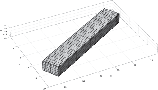
Figure 7.2 The horizontal pontoon used in the example. Quadrilateral panels as used in the 3D boundary element method.
Table 7.1 Nondimensional added mass for the pontoon shown in Figure 7.2 as computed by strip theory and at a low frequency (0.087 Hz) and a high frequency (0.5 Hz) using a 3D panel method. The added mass values are made dimensionless in the following way:
 , with
for
,
for
and
and
for
.
.
, with
for
,
for
and
and
for
.
.


| i / j | 1 | 2 | 3 | 4 | 5 | 6 | |
|---|---|---|---|---|---|---|---|
| Strip | 1 | 0.650 | -1.126 | 0.000 | -1.913 | -1.105 | -6.150 |
| 3D high | 1 | 0.871 | -0.959 | 0.000 | -1.648 | -1.448 | -5.717 |
| 3D low | 1 | 0.937 | -1.015 | 0.000 | -1.696 | -1.647 | -6.071 |
| Strip | 2 | 1.949 | 0.000 | 3.314 | 1.913 | 10.652 | |
| 3D high | 2 | 1.979 | 0.000 | 3.351 | 1.648 | 10.537 | |
| 3D low | 2 | 2.109 | 0.000 | 3.605 | 1.696 | 11.218 | |
| Strip | 3 | 6.001 | 9.002 | -27.594 | 0.000 | ||
| 3D high | 3 | 5.740 | 8.610 | -26.394 | 0.000 | ||
| 3D low | 3 | 6.381 | 9.571 | -29.340 | 0.000 | ||
| Strip | 4 | 23.637 | -45.934 | 18.108 | |||
| 3D high | 4 | 22.254 | -42.810 | 17.878 | |||
| 3D low | 4 | 24.382 | -47.567 | 19.120 | |||
| Strip | 5 | 142.260 | 10.455 | ||||
| 3D high | 5 | 134.417 | 9.749 | ||||
| 3D low | 5 | 149.038 | 10.268 | ||||
| Strip | 6 | 66.000 | |||||
| 3D high | 6 | 63.498 | |||||
| 3D low | 6 | 67.291 |
7.2.2.3 Horizontal Disks
In some cases, the substructures are equipped with horizontal plates of almost circular shape and with small thickness (as discussed in Section 4.4.1). The reason for using such plates is to tune the dynamic behavior of the platform. The plates will add inertia to the system, thus moving the natural periods in heave, roll and pitch to higher values. At the same time, plates with sharp edges will contribute to viscous damping and thus reduce the motion response in the resonant domain. To improve the damping properties, perforation of the plates is an option. A perforation will, however, reduce the added mass effect of the plate (Reference Molin and NielsenMolin and Nielsen, 2004).
The added mass of a circular disk with radius
 oscillating in infinite fluid is given by Lamb (1975, 144):
 ([7.27])
In most cases, the plate will be located at the bottom of a vertical column. In such cases the added mass will be somewhat smaller, depending upon the ratio of the disk radius to the column radius (see discussion on vertical columns in Section 7.2.2.1).
Figure 7.3 shows examples of the importance of the perforation to the added mass and linearized damping. The figures are from Reference Molin and NielsenMolin and Nielsen (2004). The nondimensional added mass and damping is presented as a function of the “porous Keulegan–Carpenter number”:
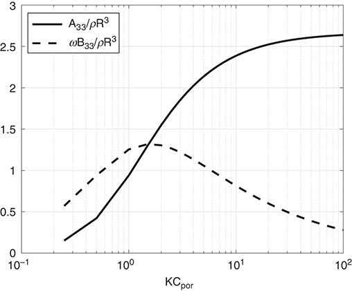
Figure 7.3 Added mass and linearized damping for a perforated disk as a function of the “porous Keulegan–Carpenter number,” KCpor. Period of oscillation 20 s, water depth 100 m, radius of disk 10 m and submergence of disk 20 m.
 ([7.28])
Here,
 is the perforation ratio (open area divided by total area of disk) and
 is the “discharge ratio”, relating the pressure drop over the disk and the relative fluid velocity through the disk. It is thus related to the flow resistance through the disk, which again is dependent upon the local geometry of the perforation.
 usually has a value between 0.5 and 1.0. Reference MolinMolin (2011) discusses various approaches to estimate the discharge ratio. It is observed from Figure 7.3 that for small
 , the added mass as well as the damping tends to zero. This case corresponds to a situation with a very large perforation area,
 . On the one hand, as
 the added mass tends toward the solid disk value of [7.27]. The computed damping tends to zero because the damping due to the edge effect of the disk is not accounted for in this theory. Including the edge effect (see Reference MolinMolin, 2011), a better agreement with the experiments is obtained for the damping.
7.2.2.4 Transformation of the Added Mass Matrix to a New Coordinate System
Frequently the added mass matrix is computed in a local coordinate system, for example, as referred to the center axis of a column or pontoon. For further analysis a different platform coordinate system may be preferred. The transformation between the two coordinate systems may be done as follows. Denote coordinates in the original (local) coordinate system by
 and the new (platform) coordinate system by
 . Assume the two systems are parallel, so that:
 ([7.29])
The kinetic energy in the fluid while oscillating the body in a certain direction must be independent of the coordinate system used. By considering the kinetic energy using the velocity potentials, it can be shown that the 6 x 6 added mass matrix in the new coordinate system,
 , is related to the added mass matrix in the original coordinate system,
 , by:
, by:
 ([7.30])
where:
 ([7.31])
Here:
 ([7.32])
Details of the derivation as well as the more general form valid also when rotations are involved may be found in Reference KorotkinKorotkin (2008).
7.3 Damping
The damping terms in [7.1] consist of several contributions that may be handled independently. The following terms will be discussed in more detail.
Viscous damping, mainly due to flow separation around the hull.
Aerodynamic damping, due to the wind turbine, and to some extent the wind forces on the tower.
Most floating structures are lightly damped. This means that the damped natural frequencies are not very different from the undamped natural frequencies. This implies that damping in most cases is important to the responses close to the natural frequencies only. However, the damping is generally both frequency-dependent and amplitude-dependent. This makes it difficult to establish accurate damping estimates. Normally, good physical insight as well as engineering experience is required to come up with realistic damping estimates. Frequently, model testing is applied to study the motion behavior of floating structures. If the tested structure is sensitive to resonant motion, model test results should be interpreted with great care as viscous damping normally is overestimated in model scale as compared to full scale.
7.3.1 Radiation Damping
Radiation damping is considered to be a linear damping contribution. For a general, rigid floating structure the damping matrix will be a full 6 × 6 matrix with frequency-dependent coefficients. To establish this damping matrix, a 3D radiation-diffraction approach is needed (see Section 6.4). A structure’s capability to generate waves is reduced if the structure is deeply submerged. This implies that a surface-piercing vertical column generally contributes more to the wave radiation damping than, e.g., a horizontal pontoon. However, in a strip theory approach, the 2D damping of a pontoon section may be applied to establish an estimate on the damping for the complete pontoon. The horizontal, normal force on the pontoon due to a harmonic motion
 normal to a section of the pontoon may be written as:
 ([7.33])
The subscript r indicates radiation damping. In [7.33] it is indicated that both the added mass and damping are frequency-dependent. The radiation effect will only account for waves radiated perpendicular to the pontoon axis. The 6 by 6 damping matrix can now be established similarly as shown for the added mass matrix. A strip theory approach accounts neither for the interaction of the radiated waves from each of the pontoon strips, nor for the interaction between the pontoons. The interaction effects may in some cases be significant for some frequencies and directions of oscillation.
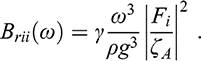
Within the context of ideal fluid flow and linear wave dynamics, there exists a reciprocity relation that relates the wave forces on a fixed body to the forces needed to oscillate the body in otherwise calm water. This is called the Haskind relation (for further discussion, see Reference NewmanNewman, 1977; Reference FaltinsenFaltinsen, 1990). The relation is valid for general 3D bodies. Applying the Haskind relation on a vertical column with a rotational symmetry, simple relations between the wave excitation forces and the diagonal of the damping matrix are obtained:
 ([7.34])
Here,
 is the wave force in direction
 ,
,
 when the waves are propagating along the
 -axis.
 for
for
 and
and
 and
and
 for
for
 . In deep water, [7.34] may be written as:
 ([7.35])
The computation of the wave force on a vertical column is addressed in Chapter 6. Note that for a substructure with several columns, there may be significant wave interaction between the columns, modifying the radiated waves and thus the damping. A summation of the damping contribution from each of the columns will thus cause errors. One should rather make a summation of the radiated wave fields, taking phases properly into account, and estimate the damping based upon the radiated energy. This is what is obtained by using 3D potential theory methods.
The Haskind relation may also be invoked to estimate the radiation damping for horizontal pontoons. Having established the wave excitation force on a segment
 of the pontoon, the corresponding contribution to the damping may be obtained. Reference NewmanNewman (1962) derived a relation between the 2D wave force and damping for a long horizontal body in deep water and beam seas. For a segment of the pontoon this relation is identical to [7.35] using
 and considering three degrees of freedom: the transverse horizontal direction, the vertical direction and rotation about an axis parallel to the body axis.
7.3.2 Viscous Damping
Viscous damping has contributions from all structural elements where flow separation occurs. Pure skin friction is in most cases so small that it may be disregarded. The viscous force is normally expressed as a quadratic quantity with respect to the relative velocity, i.e., on a short, 2D section of a vertical column, the viscous force may be written as:
 ([7.36])
Here,
 is the drag coefficient,
 is the column diameter and
 is the relative horizontal velocity between water and structure at the z-level considered.
 is the length of the short vertical section considered. It is observed that the viscous force contributes both to excitation via the
 term and damping via
 . Further, there is a coupling term between the two that contributes to damping or excitation depending upon the phase between the wave particle velocity and the motion velocity.
7.3.3 Linearization of Viscous Damping
In linear dynamic analysis there is a need for linearization of the viscous effect. This is in particular the case when accounting for viscous damping in frequency domain analyses. Due to the nonlinear nature of the damping and the coupling to the fluid velocity, i.e., wave particle and current velocities, it is in general not possible to perform a consistent linearization of the viscous damping. However, disregarding the fluid velocities and considering a single-degree-of-freedom (SDOF) system, an equivalent linear damping can be derived as follows. Consider a long slender structure, e.g., a cylinder. Denote the 2D damping force acting normal to a short section of length,
 by
by
 . The force is assumed to be composed of a linear and a quadratic contribution, i.e.:
 ([7.37])
The body velocity normal to the cylinder axis is assumed to be harmonic, i.e.,
 . To find the equivalent linear damping
 , the dissipation of energy over one cycle of oscillation,
 , is considered. By requiring the dissipated energy to be the same for the equivalent linear system and the quadratic system,
 is thus found from:
 ([7.38])
Inserting for
 and working out the integrals, the equivalent damping is obtained as:
 ([7.39])
It is observed that the equivalent linear damping is proportional to the velocity amplitude,
 . That implies that an iteration procedure usually must be implemented to establish a proper damping estimate. As the damping is of key importance to the resonant response, one will have to guess a resonant response amplitude, estimate the equivalent damping, then compute the response and correct the damping according to the computed response.
Viscous Damping
Consider the following simple 1D example. A small body is exposed to an oscillating flow given by
 . The body is moving harmonically in the same direction with a velocity
 . The relative velocity is thus given by
 . The viscous force is given from [7.36]. Considering one cycle of oscillation, the average dissipated power becomes:
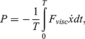
where
 . In Figure 7.4 the dissipated power is plotted as a function of phasing between the fluid velocity and the body velocity. It is observed that for cases with
 , the damping (dissipated power) is positive independent of phasing between the fluid motion and the body motion. However, for
 , the damping may become negative for certain phases, implying an excitation effect. For zero fluid velocity the average dissipated power amounts to
 .
.
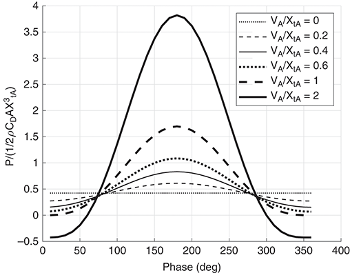
Figure 7.4 Average dissipated power as a function of phase between fluid velocity and body velocity. Amplitude ratio
 ranging from 0 to 2.
The above procedure works fine for a SDOF and in cases where the various modes of motion are uncoupled or close to uncoupled. For most substructures the heave mode has little coupling to other modes, while, for example, the surge and pitch modes may have significant coupling. Frequently the surge motion is referred to the waterline level, while the eigenmode for pitch may have a center of rotation far below the waterline. This causes a significant coupling between the surge and pitch motion when viscous drag forces are accounted for.
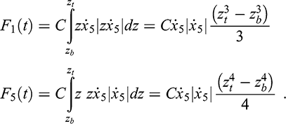
To illustrate this point, consider a spar platform designed as a vertical cylinder with constant diameter and a pure surge motion. The drag forces in surge and pitch may then be written as:
 ([7.40])
Here,
 and
and
 are the top and bottom coordinates of the cylinder.
 , with
 being the diameter of the cylinder. Computing the dissipated energy as above, the linearized damping in surge is obtained as:
 ([7.41])
Similarly, integrating the pitch moment over one cycle of oscillation and comparing the quadratic and the linear process, a linearized coupling term between the surge motion and pitch moment is obtained as:
 ([7.42])
The above approach may be repeated for a pure pitch motion, with the pitch motion referred to
 . The surge and pitch forces corresponding to [7.40] now become:
 ([7.43])
The linearized damping coefficients for the pure pitch motion are obtained as:
 ([7.44])
From the above relations it is observed that the linearized damping depends upon the choice of surge and pitch velocity amplitude used as basis for the linearization. If one focuses on a good linearization of the pitch damping at the pitch natural period, the coupling effect will cause damping also in surge that may be unrealistic. To succeed in linearization of the damping, one should aim at reducing the coupling terms in the damping matrix as much as possible. This is normally obtained by using a coordinate system in which the modes of motions are close to the eigenmodes of the system.
Viscous Damping in Coupled Motion
Consider a vertical cylinder with length equal to draft 100 m and diameter 10 m. Center of gravity is at -70 m. The 2D added mass and drag coefficients are both set to 1.0. A horizontal mooring system with stiffness 50 kN/m is attached at the waterline level. The natural periods in surge and pitch are 118.6 and 17.70 s. The pitch eigenmode has a center of rotation at z = -61.5 m. The linearized coupled damping matrix has been established by assuming a surge amplitude of 0.7 m and a pitch amplitude of 0.5 deg. The system is set into free oscillations in calm water. The initial surge amplitude is 1.0 m, while the initial pitch and all initial velocities are set to zero. Two cases are considered, one using the quadratic damping and one using the linearized damping matrix. Figure 7.5 shows the results for the two cases.
It observed that the surge motion is well reproduced using the linearized damping (upper-left), even if the surge damping force contains large contributions from the pitch motion (lower-left). Initially, the pitch motion obtained by the linearized equations follows the motions obtained by using quadratic damping well (upper-right). This is because the inertia effects dominate initially. After a while, however, the pitch motion is more and more dominated by the surge natural period in the linearized case. Large differences are also observed in the pitch drag moment (lower right).
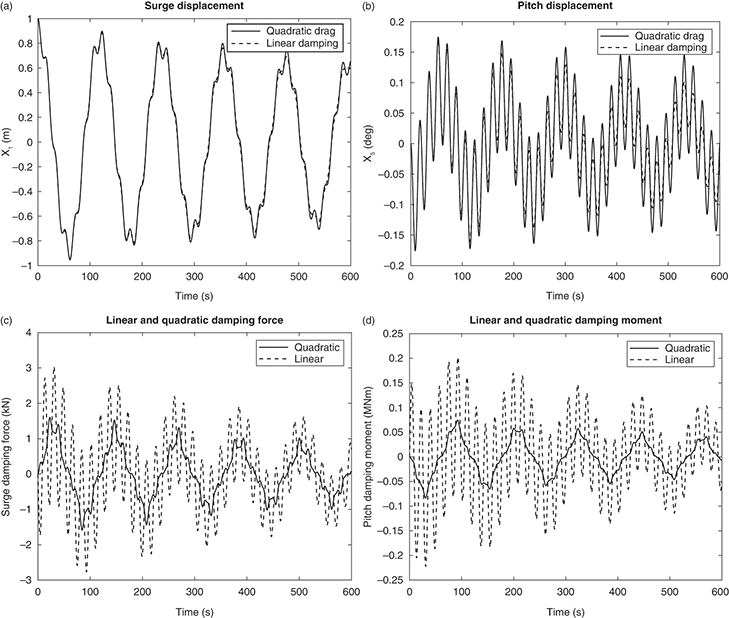
Figure 7.5 Motion decay in surge and pitch for a floating vertical circular cylinder using quadratic and linear damping. Upper figures: displacements after an initial surge of 1.0 m and zero pitch; lower figures: damping force in surge and moment in pitch.
7.3.4 The Drag Coefficient
In most practical cases, the viscous forces are related to the pressure distribution over the structure due to flow separation. That implies that the drag coefficient,
 , depends upon the body geometry, including surface roughness as well as flow conditions. The flow conditions are expressed via three nondimensional numbers: the Reynolds number,
 ; the Keulegan–Carpenter number,
 ; and the relative current number,
 . Here,
 is a characteristic flow velocity;
 is the amplitude of the oscillatory velocity, either of the body or the flow;
 is a steady current velocity;
 is a characteristic cross-sectional dimension of the body;
 is the kinematic viscosity of the fluid; and
 is the period of oscillation. Thorough discussions of the relations between these parameters and the drag coefficient are given in, e.g., Reference Sarpkaya and IsaacsonSarpkaya and Isacsson (1981) and Reference FaltinsenFaltinsen (1990). Recommended values to be used are found in, e.g., DNV (2021c).
For circular cylinders the drag coefficient is sensitive to where flow separation takes place, which again is sensitive to all the above parameters. For cross-sections with a rectangular shape, the drag coefficient is less dependent upon the flow conditions as flow separation occurs at the sharp corners. Classical results for the drag coefficient for a 2D circular cylinder in steady flow as a function of the Reynolds number are shown in Figure 7.6. A drop in the drag coefficient for the Reynolds number in the order of 105 is observed. As the surface roughness of the cylinder increases, the drop occurs at a lower Reynolds number, and is less than for a smooth cylinder.
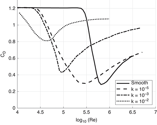
Figure 7.6 Drag coefficient for a 2D circular cylinder in steady flow as a function of the Reynolds number and surface roughness
 .
.
7.4 Wave Excitation Forces
7.4.1 Slender Bodies of General Shape
The estimation of wave excitation forces on floating substructures is now to be addressed. As for the discussion on the added mass coefficients above, structures composed of slender vertical cylinders and a horizontal pontoon using strip theory will be addressed. One of the advantages with this approach is that it is straightforward to use in a finite element analysis of the structure based upon beam elements. However, the global forces are focused upon here as these are needed for estimating the rigid-body motions. Some floating substructures may have a barge-like shape (see Section 4.4.4). To estimate the wave forces on such structures, 3D methods as discussed in Chapter 6 should be used.
As for the added mass, the forces need to be referred to a common point of reference. Further, by using the strip theory approach, it is assumed that the flow over any cross-section of the columns or pontoons may be considered to be 2D, even if the cross-sectional dimensions are changing. No hydrodynamic interaction is assumed between the various structural components.
In computing the six degrees of freedom of rigid-body wave forces, it may be convenient to refer to a coordinate system located at the mean sea surface, with
 at the surface level and positive upward.
7.4.2 Wave Forces on a Vertical Column
Consider regular waves propagating in direction
 relative to the
 -axis. The complex wave potential may, see Chapter 2, be written as:
 ([7.45])
There are two options to estimate the wave force on a vertical circular column. One may either assume a very slender column, with no diffraction effects, and apply the Morison equation or one may include diffraction effects and apply the MacCamy and Fuchs theory. Both these approaches are discussed in Chapter 6. However, the expressions need to be modified to account for the fact that the column does not extend to the sea floor. Using a strip theory approach, this implies that the sectional force is integrated from the bottom to the top of the column, i.e., from
 to
to
 .
.
 . It is assumed that the column axis is located in
 . Similarly as for the monopile, the surge and sway forces are now obtained as:
 ([7.46])
Here,
 and
and
 are given in [6.15],
 and
and
 . It is observed that the forces have an extra phase shift as the column is offset from
 . The vertical force may be estimated using the pressures from the undisturbed wave, the Froude-Krylov pressure at the bottom and top surfaces of the column, i.e.:
 ([7.47])
If the column is surface-piercing,
 , there is no wave pressure on the top end and
 . Similarly, if the column is sitting on the bottom,
 . For wetted end surfaces,
 . Note that a bottom-fixed vertical cylinder piercing the free surface is not exposed to vertical wave forces.
The moments about the
 - and
- and
 -axes are obtained similarly as in [6.15] and [6.16]; accounting for the horizontal offset, the direction of the waves and that the moment axis is now at the free surface level, the roll and pitch moments are obtained as:
 ([7.48])
The last term in the above expressions is due to the moment contribution from the vertical wave force on the column. Note that in the deep-water case,
 ,
,
 .
.
The moment around the
 -axis, the yaw moment, is obtained from the horizontal forces:
 ([7.49])
All the above expressions are valid for one single column. If several columns are present, the total force is obtained by summation over all the columns. If a column diameter is changing over the length of the column, a pragmatic approach is to split the column into, e.g., two parts and compute the force on each of the parts separately. This is illustrated in Figure 7.7. The split may be done into two or more parts. To obtain a realistic model, the body volume should be conserved. The vertical wave force at the conical part of the column may be modeled by the wave pressure at the area representing the difference between the cross-sectional area of the cylinders. The modeling of this force may be improved by representing the conical section by more cylinders.
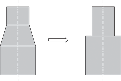
Figure 7.7 Vertical column with conical section modeled by two cylindrical sections.
If the distance between the columns is not large compared to the diameter of the columns, the interaction effect may be important. In such cases, a full 3D analysis should be performed to obtain accurate estimates on the wave forces.
7.4.3 Wave Forces on a Horizontal Pontoon
Horizontal pontoons in most cases either have a circular or a rectangular cross-section. In the case of a rectangular cross-section the added mass coefficient in horizontal and vertical directions differs. Consider the horizontal pontoon illustrated in Figure 7.8. A slender body is assumed, implying that the length of the pontoon is much longer than the characteristic cross-sectional dimension. Further, long wavelength theory is used, implying that the wavelength is much longer than the characteristic width of the pontoon. Following the principles outlined in Reference FaltinsenFaltinsen (1990), the vertical and horizontal forces on a 2D section of length
 may be written as:
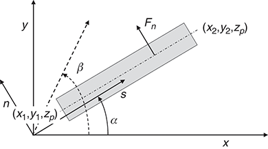
Figure 7.8 A horizontal pontoon. Notations used in deriving the wave forces.
 is the direction of the pontoon axis relative to the coordinate system used for the body.
 and
and
 are the coordinates of the end points.
 is the direction of wave propagation.
 are the local pontoon coordinates, parallel and perpendicular to the pontoon axis. The
 and
and
 planes coincide.
 ([7.50])
Here,
 is the cross-sectional area of the pontoon;
 is the 2D added mass in horizontal direction, normal to the pontoon axis;
 is the 2D added mass in vertical direction;
 and
and
 are the acceleration in the water horizontally, normal to the pontoon axis and in vertical direction respectively.
To obtain the total forces on the pontoon, the forces in [7.50] have to be integrated over the length of the pontoon. To perform this integration, it is convenient to introduce the local
 coordinates, as illustrated in Figure 7.8. The relations between the two coordinate systems are:
 ([7.51])
The coordinates of the end points of the pontoon axis are thus:
 ([7.52])
Considering a pontoon of constant cross-sectional shape, it is only the normal component of the horizontal acceleration,
 , and the vertical acceleration,
 in [7.50], that vary along the pontoon length. The horizontal acceleration perpendicular to the pontoon axis may be written as:
 ([7.53])
Integrating along the pontoon, the following result is obtained for the horizontal force on the pontoon:
 ([7.54])
In the limit
 , i.e., the waves are propagating perpendicular to the pontoon axis, the limiting value of the integral is obtained as:
 ([7.55])
If the pontoon ends are wetted, a reasonable approximation is to assume that the pressure in the undisturbed wave (the Froude–Krylov pressure) is acting on the surfaces, i.e., the force in axial direction becomes:

Here,
 for a wetted surface and zero for a dry surface. Frequently, a pontoon is attached to column of larger diameter. The end of the pontoon is then dry. On the other hand, part of the column surface is also dry. It is thus convenient to model both surfaces as wetted. This will almost cancel the global force contribution from the intersection. If local forces are required, this approach will not work.
The vertical force on the pontoon is obtained in a similar way as the horizontal force, i.e., using:
 ([7.57])
The forces in the support structure’s coordinate system
 are obtained as:
 ([7.58])
Horizontal Wave Force on Pontoon
An example of the computed horizontal force on a pontoon of length 30 m in a wave of length 15 m is shown in Figure 7.9. The force perpendicular to the pontoon axis is shown. The force is given as a function of the angle between wave propagation and the pontoon axis. By presenting the result in the format
 , the sign of the force relative to the pontoon normal axis is retained. It is observed that the extreme forces are obtained for
 . Further, zero force is obtained for waves propagating along the pontoon axis. For
 additional zero values appear. For these angles one wavelength will cover the full pontoon length, i.e.,
 .
.
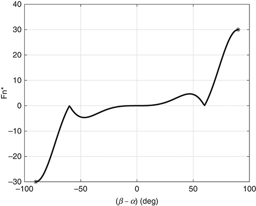
Figure 7.9 Absolute values of the wave force on a horizontal, submerged pontoon of length 30 m in a wave of length 15 m, i.e.,
 ,
,
 ,
,
 . The abscissa is the angle of wave propagation relative to pontoon axis. The force is presented as
  . The solid line is according to [7.54], while the stars are obtained using [7.55].
7.4.4 Moments Acting on a Horizontal Pontoon
Recall that the
 and
and
 planes coincide. Similar as for the pontoon forces, the moments about the
 axes may be written as:
 ([7.59])
It is observed that these expressions resemble those of the forces, with one important difference: the factor
 in the integral terms for
 and
and
 . Working out these integrals and relating them to the integrals involved in the force expressions, the moments can be written as:
 ([7.60])
Here,
 is given by:
 ([7.61])
Note that
 is complex and thus contains phase information. In the coordinate system of the support structure, the moments become:
 ([7.62])
7.4.5 Viscous Drag Effects
The viscous forces, as written in [7.36], contain the relative velocity between water and structure. For a slender vertical structure, this reads
 . Here,
 is the horizontal component of the fluid velocity and
 is the horizontal velocity of the structure. The viscous drag forces are frequently estimated using a strip theory approach, assuming the length of the structure is much larger than the characteristic cross-sectional dimension. The drag force on a strip of a vertical structural member thus becomes, assuming the fluid velocity is larger than the structural velocity:
 ([7.63])
 represents an excitation term, while the two remaining terms may represent damping, i.e., a force opposing the motion or an excitation, depending upon the phasing between the velocity components and the relative magnitude between them. In waves, the largest velocities are present close to the free surface, and the largest viscous excitation effects are thus present in this region. At greater depth, the viscous damping effect may be more important. In the above expression, the horizontal relative velocity is used to estimate the normal force. For a slender structural member of general orientation, one should use the relative velocity component normal to the axis of the member in estimating the force. This “cross-flow principle” is normally assumed to hold if the flow direction is between 45 and 90 deg relative to the member axis (DNV, 2021c). In DNV (2021c) additional recommendations on how to handle the viscous drag forces are also given. In Section 6.5.1, the viscous wave forces in the splash zone are discussed. The same effects are experienced on columns of floating structures, with the additional effect of the motion velocity of the structure.
Due to the nonlinearity of the viscous forces, time domain simulations are normally required in cases where the viscous effects play an important role in the forcing.
7.4.6 Cancellation Effects
In the design of floating support structures, the geometric layout can efficiently be utilized to minimize the wave excitation loads at certain frequencies. Consider the simple half of a semisubmersible in Figure 7.10. The half semisubmersible consists of two columns and one pontoon. It is assumed that the columns are sitting on top of the columns. Assume the waves’ direction of propagation is perpendicular to the paper plane. The undisturbed pressure in the water, the Froude–Krylov term in the wave excitation pressure, is then constant along the length of the pontoon. The vertical force acting on the semisubmersible is approximately given from the Froude–Krylov pressures acting on the top and bottom of the pontoon multiplied by corresponding areas:

 ([7.64])
Here,
 and
and
 are the wetted area of the bottom and the top of the pontoon respectively. In deep water the pressure is given from
 . Thus, the force becomes zero for a wave number
 given by:
 ([7.65])
The difference between the top and bottom areas is given from the cross-sectional area of the columns. By choosing a suitable column cross-sectional area, pontoon dimensions and submergence, a wanted wave period for cancellation may be obtained. It is observed that this expression also holds if the platform consists of two parallel pontoons. In the case of two parallel pontoons, there will also be a close-to-zero vertical excitation force if the distance between the pontoons is half a wavelength. However, as the zero vertical force corresponds to a wavelength about half the distance between the pontoons, this wavelength will cause a maximum in the roll motion of the structure.
Consider waves propagating in the paper plane (Figure 7.10). If the wavelength is approximately twice the distance between the columns, the horizontal acceleration in the wave acting on the two columns will have opposite phase. Thus, a close-to-zero horizontal excitation force is acting on the platform. It should be noted that wavelengths that correspond to close-to-zero wave excitation forces on the complete structure in many cases correspond to the wavelengths giving the largest internal forces in the structure. This is easily understood by considering the case of opposite phase of the forces on the two columns.
For the spar platform, the lower part of the hull is normally designed with larger diameter than the diameter at the water line (see Figure 7.7). This difference in diameter is required to ensure a sufficient buoyancy while at the same time keeping the natural frequency in heave below the range of wave frequencies. As for the pontoon, the vertical excitation force may be approximated by the Froude–Krylov force on the bottom of the spar minus the vertical component of the Froude–Krylov force acting on the conical part, simplified as illustrated in Figure 7.7 (right). Thus, a cancellation effect of the vertical wave force is obtained for a certain wave frequency. In principle it is possible to design both a semisubmersible and a spar to have a cancellation frequency at the heave natural frequency. Theoretically, this could significantly reduce the resonant motions. However, due to other design requirements, this option is not used in practical design.
7.4.7 Wave Forces on Large-Volume Structures: Boundary Element Method
The basic principles for the 3D boundary element method are outlined in Section 6.4. In Table 7.1, the added mass and damping for a horizontal pontoon as computed by strip theory and a 3D boundary element method are compared. In the below example the corresponding wave excitation forces are compared.
One may question why strip theory approaches should be used when full 3D tools are available. There are several reasons for this. Strip theory is much faster, both in establishing the numerical model and performing the computations. This feature makes the method well suited for use in optimization tools. Further, it is easy to identify the added mass and excitation force components related to the various structural components. Further, strip theory is ideal for implementing hydrodynamic forces into a program for global structural analysis of the foundation as the sectional forces are readily available. However, the 3D boundary element technique is superior in computing the hydrodynamic loads for complex structures accounting for interaction phenomena between the various structural components.
Wave Forces on a Horizontal Pontoon
The horizontal pontoon used in the example in Section 7.2.2.2 is considered. The wave forces are computed both using strip theory, using the added mass coefficients from the previous example, and using the 3D boundary element method.
The draft and orientation of the pontoon is as before. Water depth of 100 m is assumed. The waves are propagating in positive
 -direction. The real and imaginary part of the wave forces in the six degrees of freedom as a function of frequency is obtained as displayed in Figure 7.11. The solid lines are the real part of the forces as computed by strip theory; the dashed lines are the corresponding imaginary part. The dots and crosses are the results from the 3D boundary element method. The forces are scaled by a factor
 for the linear forces.
 is the wave amplitude. The moments, computed around origin, are scaled by
 .
.
A clear cancellation effect is observed for modes 1–3 around 0.25 Hz, corresponding to a wavelength of about 26 m, which is the projected length of the pontoon in the direction of wave propagation.
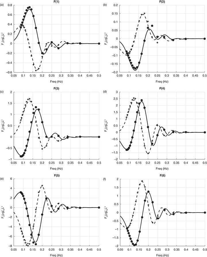
Figure 7.11 Real and imaginary part of the wave excitation forces on the horizontal pontoon shown in Figure 7.2.
7.4.8 Time Domain Simulations with Frequency-Dependent Coefficients
As briefly mentioned in Section 7.1, the hydrodynamic added mass and damping coefficients are frequency-dependent. The frequency dependency of the added mass is frequently ignored if the structure is slender or deeply submerged (see discussion of the Morison equation versus the MacCamy and Fuchs solution in Chapter 6). The frequency dependence of the hydrodynamic coefficients is related to body’s capability to generate waves when oscillating. Thus, there exists a relation between the frequency-dependent part of the added mass and the wave radiation damping.
One of the attractive properties of the linear formulation of the hydrodynamic coefficients and excitation forces is the option of solving the equations of motion in the frequency domain. However, even if it may be justified to linearize the hydrodynamic problem, that may not be the case for other parts of the problem such as the aerodynamic loads. The equations of motion for the complete floating wind turbine must thus be solved in time domain. This requires special attention to the frequency-dependent added mass and damping. The problem was addressed by Reference CumminsCummins (1962) and Reference OgilvieOgilvie (1964). Reference FalnesFalnes (2002) and Reference Næss and MoanNaess and Moan (2013) also discuss how the frequency-dependent hydrodynamic coefficients may be transferred to time domain. In time domain, the linear equations of motion may be written (the “Cummins equation”) as:
 ([7.66])
 is known as the retardation function or the impulse response function. The equation is obtained by a Fourier transform of the linear equations of motion in frequency domain:
 ([7.67])
The added mass and damping coefficients are spit into a constant and a frequency-dependent term,
 and
and
 . Here, the index
 denotes the asymptotic value as the frequency tends to infinity. For a stationary body, i.e., a body with zero mean forward speed,
 , no waves are created as the frequency of oscillation tends to infinity. The integral term in [7.66] may be regarded as a memory effect, as it contains information of all past time. It may be assumed that the body is as rest for
 . Further, the causality condition is invoked, i.e., the system cannot react upon future forces. Utilizing symmetry properties of
 and
and
 , and the requirement that
 must be real, it can be shown that the retardation function can be written on two different forms, using either the radiation damping or the frequency-dependent part of the added mass:
 ([7.68])
These expressions also show that the damping and the frequency-dependent part of the added mass are both related to the body’s ability to radiate waves when oscillating. More details upon these issues are found in Reference FalnesFalnes (2002). In principle, it is thus straightforward to obtain the retardation function if the frequency-dependent added mass or damping are known, e.g., from a boundary element panel code analysis. However, such codes have issues related to so-called “irregular frequencies” (see Section 6.4) and low accuracy as the wavelength approaches the size of the panels. Thus, to establish the high-frequency limit of the added mass may involve some challenges. For further discussion of these issues, see Reference FaltinsenFaltinsen (2005).
The convolution integral in [7.66] may be costly to evaluate, in particular for long simulations and thus large
 . In practical simulations the integration is truncated. The memory effect is assumed to negligible after some finite time. Various ways to speed up the evaluation of the convolution integral for implementation in state-space simulation models have been suggested. Reference Duarte, Alves, Jonkman and Sarmento.Duarte et al. (2013) compare several methods for approximating the retardation functions and discuss accuracy as well as computational speed.
Figure 7.12 gives examples of the frequency-dependent radiation damping and the corresponding retardation functions. The structure considered is a spar platform with shape as given in Figure 6.10. For such a geometry, it is straightforward to obtain an accurate estimate of the radiation damping. For a semisubmersible with a more complex geometry, this is more demanding. It is observed that the retardation functions as shown in Figure 7.12 tend to zero after a few oscillations. After approximately 30 s, the retardation functions are approximately zero and the memory effect has vanished.
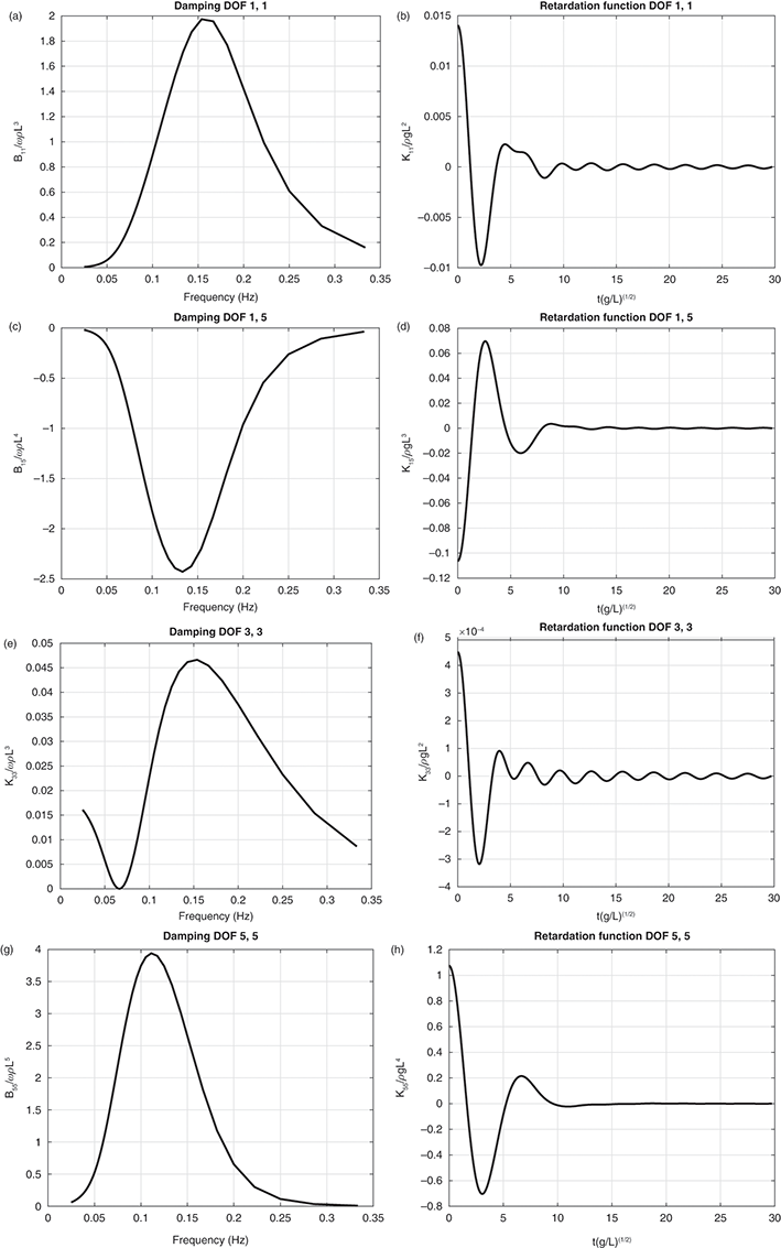
Figure 7.12 Radiation damping for a spar platform with draft of 76 m and maximum diameter of 14.4 m (see Figure 6.10). Left: damping in surge, heave, pitch and coupled surge-pitch; right: corresponding retardation functions. Length parameter used for scaling,
 .
.
7.5 Restoring Forces
7.5.1 Hydrostatic Effects
The restoring forces acting on a floating wind turbine substructure are due to the hydrostatic effects and the mooring lines. The hydrostatic forces are, for normal motions, assumed to be linear. The 6 x 6 hydrostatic stiffness matrix may be written as:
 ([7.69])
Here,
 is the mass of the body;
 is the submerged volume of the body;
 is the CG of the body;
 is the volume center of the submerged body (center of buoyancy, CB);
 is the water plane area;
 are the first moments of the water plane area,
 are the second moments of the water plane area;
 and
and
 . The hydrostatic stiffness matrix is symmetric. For a freely floating body
 and
and
 , several of the off-diagonal terms in [7.69] thus become zero. This is, however, not the case if the static mooring forces are significant as compared to the buoyancy force. It is assumed that
 is a rigid mass, i.e., there is no fluid that may move inside the body.
7.5.2 Effect of Catenary Mooring Lines
The geometry and loads in catenary mooring lines are discussed in Section 7.6. The restoring forces are generally very dependent upon the pretension and offset of the top end of the mooring line. However, given a certain position of the top end, the linearized contribution to the stiffness matrix from each of the mooring lines may be computed as follows.
Initially the line is assumed to give restoring effects resulting from motion in the plane of the catenary only. The catenary line is assumed to be located in a local
 plane with origin in the upper end of the mooring line. The 3 x 3 restoring matrix for each line
 has thus only the following non-zero elements:
 . The local plane is rotated an angle θ about a vertical axis relative to the global coordinate system. The restoring force matrix in a coordinate system parallel to the substructure’s coordinates then becomes:
 ([7.70])
Here, the transformation matrix due to the rotation about the
 -axis is given by:
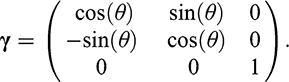 ([7.71])
The line is supposed to be attached to the support structure at
 in the substructure’s coordinate system. The 6 x 6 stiffness matrix referred to the substructure becomes then:
 ([7.72])
with the
 given by:
 ([7.73])
Mooring System Stiffness
As an example, we may consider the stiffnesses in surge, heave and pitch for a mooring system consisting of three symmetrically spaced mooring lines (
 ). We then obtain the following contributions to the restoring matrix for the platform:
 ([7.74])
The last expression at each line corresponds to the result for the symmetrical three-point mooring.
 is the azimuth angle of the mooring line attachments as referred to the platform coordinate system,
 is the vertical coordinate of the mooring line attachments and
 is the radius of mooring line attachments, i.e.,
 . The contribution from
 and
and
 becomes zero in this symmetrical case.
7.5.3 Effect of Tether Mooring
Tether mooring systems normally consist of one or more vertical lines with pretension (see Chapter 4). The pretension level is governed by the design requirement that the line should never go slack. Tether mooring has for a long time been applied on offshore oil and gas platforms. The advantage of using tether mooring is that the heave, roll and pitch motions are all very small, i.e., restrained modes. In the oil and gas industry, this has opened up the option of having dry well-heads on a deck of floating platforms. Tether mooring is normally combined with a hull design that minimizes the dynamic wave loads in the tethers. In contrast to catenary mooring lines, tether mooring implies permanent vertical loads on the anchors. This calls for special anchor designs, for example, bucket or gravity anchors with a submerged weight at least equal to the pretension in the tether.
A challenge using multiple tethers (three or more) for floating wind turbines is the large overturning moment due to the wind thrust on the turbine. This overturning moment is
 , where
 is the wind thrust and
 is the vertical distance between the rotor axis and the point of attachment of the tethers. Using four tethers in a square layout as an example, the force in each of the tethers to compensate for the overturning moment amounts to
 . Here
 is the distance between the tethers. Thus, the dynamic loads in the tethers increase with the
 ratio. For most wind turbines
 , implying large dynamic load variations in the tethers as compared to the dynamic wind thrust. This put requirements to the pretension in the tethers which again may be a driver for the buoyancy of the substructure and the size of the anchors.
The 3 x 3 (surge, sway, heave) restoring matrix for one single tether, referred to the top end of the tether, is:
 ([7.75])
Here,
 is the tether tension,
 is the tether length and
 is the axial stiffness per unit length of the tether. Using [7.72] and [7.73] to transfer this stiffness matrix to the platform origin, the symmetrical 6 x 6 restoring matrix becomes:
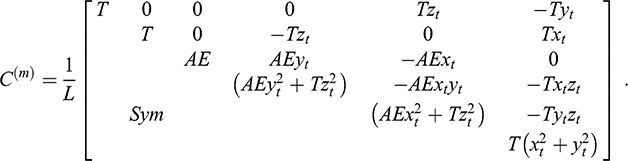 ([7.76])
7.6 Mooring Lines
The main purpose of a conventional mooring system is to keep the floating structure at location, i.e., to avoid drift-off due to mean forces from wind, waves and current. Except for tether systems, used for tension leg platforms, mooring systems are normally not designed to restrict the dynamic wind and wave forces. A mooring system should thus be sufficiently strong to take the maximum average plus slowly varying forces, and at the same time sufficiently compliant to avoid extreme loads due to dynamic offset. The force-displacement characteristics of mooring lines are normally very nonlinear, as illustrated in Figure 7.13, which shows how a certain horizontal mean force (in this case approximately 2400 kN) corresponds to a certain static horizontal offset of the top end of the mooring line (fair lead). In this specific example the fair lead position is offset by approximately 620 m from the anchor position. Adding wind- and wave-induced horizontal motions on top of the mean offset, the corresponding mooring line tension will vary according to the nonlinear force-displacement characteristic. It is observed that if the mean force increases, the tension amplitude corresponding to a certain motion amplitude will increase.
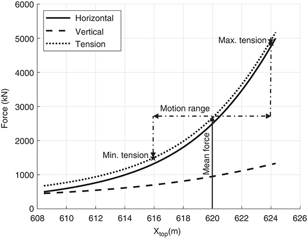
Figure 7.13 Force-displacement characteristic for a mooring line of length 627.0 m in unstretched condition. The top end is located 71.2 m above the sea floor. Submerged weight per unit length is 2.46 kN/m. The axial stiffness EA = 892.6 MN. The
 -axis gives the horizontal distance from the anchor location to the top end (fair lead). The vertical arrow indicates a mean load in the line and the corresponding mean distance from the anchor. The dot-dashed horizontal line indicates a double amplitude of wave- and wind-induced motions, causing the tension in the line to vary between the values given by the stars.
To avoid excessively large extreme load amplitudes and to ensure that the anchor can withstand the loads, it is normally required that the length of the mooring line shall be sufficient to ensure that the mooring line force at the anchor position acts as a purely horizontal force, even during extreme load cases.
The pretension is important to ensure a proper stiffness in yaw for a floater. In the case of a vertical-axis wind turbine (VAWT) the mooring system must also resist the generator torque. This puts special design requirements on the mooring system. If a VAWT is placed on top of, e.g., a spar platform, and the mooring lines initially have a radial pattern, the torque will cause a rotation of the foundation until the mooring line tension component in the circumferential direction balances the generator torque. At the same time the turbine mean thrust load must be carried by the lines.
7.6.1 The Concept of Effective Tension
Before discussing the geometric and restoring characteristics of mooring lines, the concept of “effective tension” will be explained.
Hydrostatic forces arise due to the pressure acting on the surface of a body. The total hydrostatic force vector is given by integrating the pressure over the wetted surface:
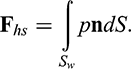 ([7.77])
Here,
 is the wetted area of the body and
 is the unit surface normal vector. If the body is fully submerged (or surface-piercing, with zero pressure at the free surface), the surface fully encloses the volume of the body. In that case the surface integral can be rewritten to a volume integral by observing that the hydrostatic pressure is given from a potential field, and invoking the Gauss theorem, i.e.:
 ([7.78])
Thus, a purely vertical buoyancy force is obtained. In the case of the cable and considering a short segment, the segment is not wetted at the end surfaces. Thus, the volume integral does not describe the hydrostatic effect and must be corrected for missing pressure at the end surfaces. This correction is illustrated in Figure 7.14. The buoyancy force is applied as if the end surfaces are wetted, i.e., [7.78] is used. Next, the forces on the end surfaces are corrected to compensate for the missing hydrostatic pressure. This introduces an additional axial tension amounting to
 . This is not a physical tension creating stress in the line, but a correction term entering the equations for the equilibrium of the line. Thus, in computing the axial tension in computing the line geometry, the effective tension is to be used:

 is the tension as obtained using the forces acting at the ends of the line and a submerged weight per unit length as given by
 . In [7.79] the hydrostatic pressure is denoted
 to show that this is an external pressure. For pipelines, a similar correction is obtained considering the effect of the internal pressure.
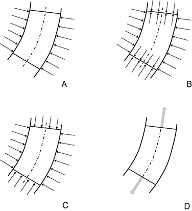
Figure 7.14 Illustration of the effective tension concept for a short segment of length
 . Case A shows the real pressure distribution. Case B gives the same net forces as Case A. Case B may be replaced by Case C plus Case D. Case C represents a fully wetted segment with vertical force
 . The end forces in Case D are the needed correction forces,
 .
.
 is the cross-sectional area of the line and
 is the external hydrostatic pressure.
Assume the line segment has a length
 at zero tension. Under tension the length is
 . The strain is then given by
 . However, also the external pressure influences the axial strain of the segment. For a cylindrical body exposed to external pressure
 on the sides and an axial tension
 , the linear axial strain is obtained as:
 ([7.80])
Here,
 is the Young’s modulus of elasticity and
 is the Poisson’s ratio,Footnote 1 which are both material-dependent. Small strains are assumed, and thus a linear stress-strain relation may be assumed. For steel within the elastic range of deformation the Poisson’s ratio is approximately 0.3, while for synthetic ropes it is close to 0.5. A Poisson’s ratio of 0.5 implies that the line, within a first-order approximation, conserves the volume when tensioned. If the Poisson’s ratio is less than 0.5, the volume increases when the line is tensioned. If it is assumed that
 is a reasonable value for the mooring line, it is observed that the axial elongation may be computed using the effective tension and disregarding the Poisson effect:
 ([7.81])
For mooring lines, the effective tension concept does not change the forces significantly. For larger-diameter structures, however, the effect is very important. E.g., deep-water pipelines may experience axial compression forces in the wall. However, they will not buckle as the effective tension is positive.
7.6.2 Inelastic Catenary Line
The static equilibrium equations for mooring lines are derived under the assumption of no bending stiffness in the line and small axial elongations. In the following, the axial elongation is ignored. Consider a line suspended between two points, A and B, as shown in Figure 7.15. The line has a length
 and it is assumed that the line is submerged in water. The vertical forces acting are the weight and the buoyancy,
 . Here,
 is the weight in air per unit length of the line and
 is the mass per unit length.
 is the density of water and
 the cross-sectional area. No horizontal forces are acting along the line; the horizontal component of the tension in the line
 is thus constant along the line. At each end of the line, vertical and horizontal point forces are acting.
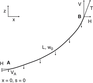
Figure 7.15 Forces acting on a line with constant weight per unit length suspended in water between Points A and B.
Consider a small section,
 , of the line, as illustrated in Figure 7.16, and consider equilibrium in the tangential and normal direction of the line:
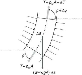
Figure 7.16 Forces acting upon a short segment of the line.
 ([7.82])
Here, the variation of the external pressure over the segment has been ignored. Using
 ,
,
 and
and
 and letting the segment length tend to zero, [7.82] is rewritten as:

The
 and
and
 derivatives with respect to the line coordinate are obtained as:
 ([7.84])
By integrating these equations, the so-called “inelastic” catenary equations are obtained:
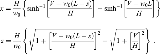 ([7.85])
Here,
 are the coordinates of the line with
 at the upper end (B) where
 .
.
 and
and
 at the lower end (A). Further details of the derivation of the catenary equation can be found in Reference FaltinsenFaltinsen (1990) or Reference TriantafyllouTriantafyllou (1990). Reference FaltinsenFaltinsen (1990) also shows how one may account for the fraction of the line resting upon the sea floor.
7.6.3 Elastic Catenary Line
For mooring line applications, the elastic elongation of the line may be of importance, even if it is assumed to be small. A first-order approximation of the elastic effects is thus acceptable. The stretched length of the segment in Figure 7.16 is
 , with
 . Assuming the Poisson’s ratio
 , the volume of the segment will not change under the action of tension or external pressure. Thus, the buoyancy force acting upon the tensioned segment is equal to that of the unstretched segment,
 . The equations for the balance between horizontal and vertical forces on a line segment are thus similar as for the inelastic line, accounting for the new segment length:
 ([7.86])
The
 and
and
 coordinates of the stretched line are obtained from:
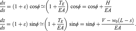 ([7.87])
Integrating as for the inelastic equations, the elastic catenary equations are obtained, assuming small linear strain and conserved volume:
 ([7.88])
For further discussion and details, see Reference TriantafyllouTriantafyllou (1990).
7.6.4 Restoring Characteristics
As an example, the mooring line described in Figure 7.13 is used. Static force-displacement characteristics in the plane of the catenary are considered. This technique is valid for static loads and slow motions only. As the speed of the motion increases, or the frequency of oscillation increases, viscous forces acting upon the line become important and modify the restoring characteristics. This effect is discussed in more detail below.
The line configurations for various horizontal tension levels are shown in Figure 7.17. Note the large changes in touch-down position even for small changes in position of the fair lead (top end). Changing the horizontal force from 50 kN to 4500 kN moves the fair lead by 41.4 m. The corresponding change in touch-down position is 425.1 m. The elastic elongation of the line is only 0.51% at the largest tension level, i.e., the line length increases from 627.0 m to 630.2 m.
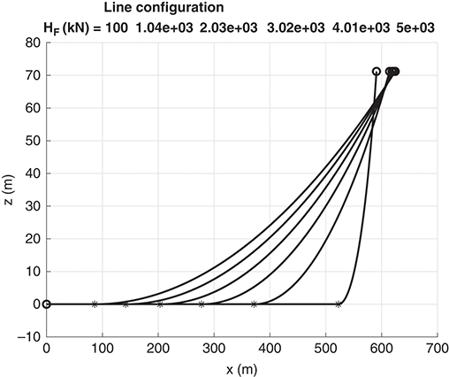
Figure 7.17 Static configuration of the line described in Figure 7.13 for various horizontal force (HF) levels. The stars denote the points of bottom touch-down, while the circles show the anchor and fair lead positions. For the case with H = 3020 kN, the touch-down is at 203.4 m. The horizontal distance from anchor to fair lead is 621.1 m, and the length of the line between touch-down and fair lead is 424.3 m (both lengths referred to in unstretched condition. For a horizontal tension of 3020 kN, the line stretches by 0.34%).
The force-displacement characteristic of a mooring line is in most cases related to the change in geometry of the line, not the elastic elongation. As seen from Figure 7.17, even small horizontal displacements at the top end of the line cause large transverse motions of the line. This is a very important effect in the case of dynamic excitation of the mooring line.
Figure 7.18 shows the restoring coefficients as a function of the horizontal force level. The restoring coefficients are defined as
 ,
,
 ,
,
 . The stiffness is largest in the horizontal direction,
 , and increases in this case almost linearly with the horizontal force. The vertical stiffness,
 , is only a small fraction of the horizontal stiffness. The coupling stiffness,
 , is also significantly less than the horizontal stiffness, but it is worth noting that a horizontal displacement may cause a significant vertical force.
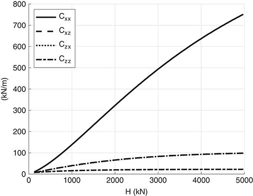
Figure 7.18 Restoring coefficients for the mooring line described in Figure 7.13 as a function of horizontal force (HF) level.
For further discussion it is useful to consider the mooring line stiffness composed of two contributions in a series coupling. The two contributions are the geometric stiffness effect and the elastic stiffness. The elastic stiffness,
 , is due to the elasticity of the line, i.e.,
 ; the geometric stiffness,
 , is the stiffness due to the force-displacement relations found from the inelastic catenary equations, [7.84]. The total stiffness may be written as
 .
.
For low tension levels, the geometrical change is relatively large even for a small change in force, as illustrated in Figure 7.17. In this force range the geometric stiffness thus dominates the total stiffness. As the tension level increases, the geometric changes are reduced. This is in particular the case if the touch-down point has moved all the way to the anchor. The geometry then approaches a straight line and the stiffness asymptotically approaches the elastic stiffness. This is illustrated in Figure 7.19.
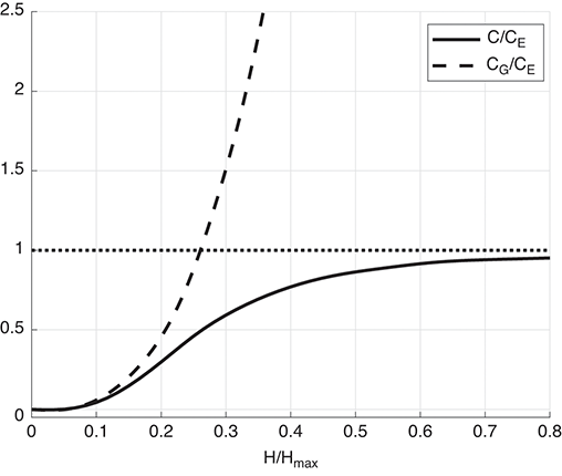
Figure 7.19 Illustration of the relative importance of the elastic and geometric stiffness as a function of the horizontal force level.
7.6.5 Dynamic Effects
From the above discussion it is observed that a small displacement of the top end of the line may cause large transverse displacements along the line. If the top-end displacement takes place at a finite velocity, as in an oscillatory motion, drag forces will act along the line. Considering a small segment of the line of length
 , the local transverse and tangential drag force along the segment may be written as:
 ([7.89])
These forces will oppose the change of line geometry. The top-end force will thus be larger than in the static case. To solve this force-displacement relation in the general case, including the above viscous drag forces as well as inertia effects, a time-domain finite element approach is required. However, it is possible to establish some estimates to illustrate the effect of the viscous forces. For this purpose, it is assumed that the line may be modeled as an elastic catenary with homogeneous properties, and the elastic deformations are assumed to be much smaller than the geometric deformations.
The line configuration, together with the notations used, are shown in Figure 7.20. The motion of the line, relative to the initial static equilibrium configuration, is denoted
 , with normal and tangential components
 and
and
 . It is assumed that the motion tangential to the top end is dominating the deformation of the line, while top-end motion normal to the line is of minor importance.
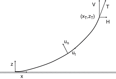
Figure 7.20 Line configuration used for the simplified dynamic analysis.
At the initial configuration, the line has a top tension
 . By adding a top tension
 , the elastic additional deformation of the top end,
 , is obtained by integrating the strain along the full length of the line:

Here, the index
 refers to the value at the top,
 . The geometric contribution to the top-end tangential displacement is thus
 , where
 is the total top-end displacement. The corresponding static displacements along the line are denoted
 and
and
 . It is now assumed that the dynamic displacement along the line is proportional to the static displacement, i.e., the geometric dynamic displacement can be written as:
 ([7.91])
If the top-end motion is assumed to be harmonic and the drag forces are linearized,
 becomes a complex coefficient relating the quasi-static geometric displacements and the dynamic displacements. The velocities and accelerations along the line are thus given by:
 ([7.92])
The normal and tangential dynamic loads acting along the line may be written as:
 ([7.93])
Here,
 is the density of the water;
 is the drag coefficient for flow normal to the line; d is the diameter of the line;
 is the mass per unit length;
 is the added mass coefficient normal to the line; and
 is the longitudinal drag (skin friction) coefficient. No added mass is included in the tangential direction. There must be a balance between the dynamic forces along the line, as expressed by [7.93], and the end forces acting on the line. It is convenient to consider the moment of the forces about the touch-down point. The moment of the distributed dynamic forces may be written as:

Here,
 is the angle between the tangent of the line and the horizontal plane. Similarly, the moment due to the top-end forces minus the quasi-static contribution may be written as:
 ([7.95])
 is the quasi-static top-end force. The difference between the dynamic and the quasi-static top-end force is given by the differences in the top-end strain,
 , i.e.:
 ([7.96])
As it is assumed that the dynamic displacement is following the quasi-static mode shape, there will be proportionality between the strain at the upper end and the elastic displacement along the line. Thus, the following relation is obtained between the top-end strain and the top-end elastic displacement:
 ([7.97])
The above equations may now be solved by requiring
 .
.
 is obtained as:
 ([7.98])
As
 depends upon
 , an iteration procedure must be used to solve for
 . The total dynamic top tension, including the quasi-static contribution, may be written as:
 ([7.99])
As both drag and inertia forces are acting on the line, there will be a phase shift between maximum force and maximum displacement. An “apparent stiffness” and damping force for the line may be derived. In very slow oscillations,
 will be close to unity and the dynamic tension variation will be close to the quasistatic value. As the drag forces on the line increase, either due to a higher frequency of oscillation or due to a larger oscillation amplitude,
 will decrease and the dynamic tension will increase. This effect is called “drag-locking” as the drag forces restrict the transverse motion of the line and force shifts the deformation from a geometric to an elastic deformation. The apparent line stiffness thus increases.
If the assumption of a quasi-static deformation pattern of the line is to be reasonable, the frequency of oscillation should be significantly lower than the lowest natural frequency of the line. A rough estimate of the natural frequencies for transverse oscillation may be obtained by using the natural frequencies of an elastic horizontal line with sag and fixed at both ends, as illustrated in Figure 7.21. The horizontal force is
 and the sag at the mid-span
 . The sag is assumed to be much less than the length of the line, causing the chord-length,
 , to be approximately equal to the line length and the horizontal force approximately equal to the line tension. Under these assumptions, the two first natural frequencies are obtained as:
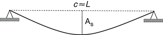
Figure 7.21 Horizontal elastic line with sag, and axial stiffness
 .
.
 ([7.100])
Here,
 is the added mass per unit length for transverse oscillations. The first natural frequency corresponds to a half-sine mode along the span. It therefore involves axial deformations. The second natural frequency corresponds to a full sine mode and does not involve axial deformations.
Dynamic Amplification of Line Tension
Consider a catenary line of length 600 m and with homogeneous mass and stiffness properties. Further details are specified below.
| Line weight | 290 N/m |
| Vertical distance from sea floor to fair lead | 60 m |
| Axial stiffness (EA) | 610 MN |
| Line mass | 34.0275 kg/m |
| Line diameter | 0.07 m |
| Added mass coefficient (normal) | 1.0 |
| Drag coefficient (normal) | 1.0 |
| Drag coefficient (tangential) | 0.05 |
| Horizontal force | 777.55 kN |
| Results from static analysis: | |
| Vertical force, top of line | 165.30 kN |
| Total top force | 794.93 kN |
| Stretched length of line | 600.77 m |
| Top-end angle | 12.00 deg |
| Horizontal position of touch-down | 29.04 m |
| Horizontal stiffness, Cxx | 272.81 kN/m |
| Vertical stiffness, Czz | 1.395 kN/m |
| Coupled stiffness, Czx | 28.69 kN/m |
| Elastic stiffness, EA/L | 1016.67 kN/m |
| Length of secant (touch-down–fair lead) | 570.68 m |
| Angle of secant | 6.00 deg |
| Line sag | 14.86 m |
The two lowest transverse natural frequencies are estimated at 1.01 and 1.58 rad/s respectively. Figure 7.22 shows the dynamic amplification of the top tension as a function of oscillation frequency for two top-end tangential motion amplitudes,
 0.1 m and 0.45 m. The results are compared to results from a nonlinear time-domain finite element program (FEM) using the Morison equation for the hydrodynamic forces (Reference Ormberg and BachynskiOrmberg and Bachynski, 2012).
Based upon the above estimates of the natural frequencies, one may expect the results to be valid for frequencies well below 1 rad/s only. The importance of the drag forces diminishes as the amplitude of oscillation is reduced. For the 0.1 m amplitude it is observed that the dynamic load amplitude is lower than the quasi-static amplitude in the low-frequency range. This is explained by the effect of the inertia loads, acting in opposite phase to the restoring force.
For the largest amplitude, the drag forces are more important and a more rapid increase in the dynamic tension is observed as the frequency increases. As the frequency of oscillation increases, the difference between the present simplified approach and the FEM results increases. An important reason for this is the assumption of a motion pattern similar to the quasi-static deformations. The somewhat irregular look of the FEM results is due to irregularities in the time-domain results causing difficulties in identifying the relevant amplitudes of the dynamic loads.

7.7 Low-Frequency Wind-Induced Motions
As discussed in Chapter 2, several methods exist for generating the point spectra of the wind velocity and the coherence of the wind field. Few measurements are available to validate the various methods, in particular for heights beyond 100 m above sea level and for the horizontal coherence. Frequently, the models applied assume neutral stability of the atmosphere. As discussed in Chapter 2, atmospheric conditions with almost neutral stability are not the most common situation. The uncertainty about relevant spectral models and coherence functions is significant in the low-frequency range. Therefore, great care should be exercised in the choice of wind field model when studying the dynamic response of floating wind turbines.
Reference Nybø, Nielsen and GodvikNybø, Nielsen and Godvik (2022) used various models to generate the wind field and studied the low-frequency dynamic response of a 15 MW offshore wind turbine on a spar floater. The rotor diameter is 240 m and the height of the rotor center is 135 m above sea level. The natural periods for the rigid-body motions (surge, sway, heave, roll and pitch) for this kind of floaters may be in the range of 25–200 s. This range of periods is normally not considered important for bottom-fixed wind turbines. Depending upon the technique used to generate the wind field, large differences in energy and coherence may appear in this low-frequency range. This is particularly the case in non-neutral atmospheric stability conditions. For the lowest frequencies it may be questioned whether the frequency content is part of a stationary process or due to nonstationarity of the wind conditions. Independent of the cause, the result may be excitation of low-frequency motion modes.
Reference Nybø, Nielsen and GodvikNybø et al. (2022) used four different wind field formulations for the response analyses: the standard Kaimal spectrum with an exponential coherence model; the Mann spectral tensor model; a wind field generated by Large Eddy Simulation (LES) code; and a model using a wind spectrum based upon measured wind speed time series combined with a Davenport coherence model fitted to wind speed measurements at two different vertical levels. This wind field is called TIMESR. The LES wind field and the TIMESR both account for atmospheric stability in the coherence, while the Kaimal and the Mann implementations assume neutral stability. However, the turbulence intensity and mean wind shear are in these two models fitted to measured data. Thereby, the mean wind speed, turbulence intensity and wind shear are similar in all the applied models. In particular in the low-frequency part, below 0.1 Hz of the spectra, significant difference in the energy content is observed between the four methods. This is illustrated in Figure 7.23. It is observed that the power spectra density (PSD) of the LES spectrum is significantly lower than what is obtained by the other three methods. The coherence computed from the wind fields also differs greatly. These differences are important for the excitation of the various rigid modes of motion.
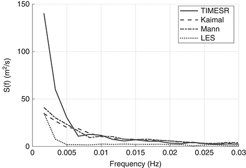
Figure 7.23 Power spectral density (PSD) in the low-frequency range of the wind spectrum calculated by four different methods. Neutral atmospheric stability and 13 m/s mean wind speed are assumed.
In Figure 7.24 illustrations of the importance of coherence to the excitation loads are given. Case A illustrates large coherence in vertical direction over a length scale similar to the rotor diameter, i.e., the dynamic wind speed is in phase over this length scale. In the horizontal direction, the coherence is assumed to be lower, causing opposite phase of the wind speed between the two sides of the rotor disk. In Case B, the length scales of the vertical and horizontal coherences have switched, i.e., large coherence in horizontal direction is assumed, while in the vertical direction the wind speed has opposite phase in the lower versus the upper part of the rotor. In Case C, the flow is assumed to be coherent over most of the rotor disk, while in Case D, the turbulent structures are assumed to have very short extent giving a very low coherence over the rotor disk area both in the vertical and the horizontal direction.
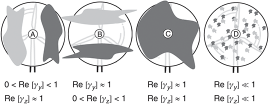
Figure 7.24 Illustration of different coherent structures that give different excitation of the various modes of motion. Dark- and light-gray tones indicate areas where the dynamic wind speed is out of phase.
As indicated in the table in Figure 7.24, the three cases will excite the different modes of motion differently. Case C will cause the largest excitation in surge, while Cases A and B will cause lower loads as the total load on the rotor disk is partly canceled out due to the phase differences. The same argument can be used for the platform pitch motion, referred to the water line and the mooring loads. For the yaw motion, however, it is observed that Case A will excite this mode more severely than Cases B and C. Which case is most relevant is obviously dependent upon frequency and rotor diameter considered. To which extent the atmospheric stability and height over sea level change the structure of the coherence is a topic for ongoing research.
Figure 7.25 shows examples of the results obtained by Reference Nybø, Nielsen and GodvikNybø et al. (2022). The standard deviations of the surge, pitch and yaw motions in 7, 13 and 18 m/s mean wind speed are given. Further, the damage equivalent load (DEM) for the most heavily loaded mooring line is given. The DEM is an expression for the fatigue loading in the line. The four wind spectra discussed above are used and neutral atmospheric stability is assumed. The turbulence intensity is in the range of 2–6.6%. From the figure it is observed that there is a large scatter between the results as obtained by the different methods for generating the wind fields. The spectra obtained by TIMESR contain much energy at the lowest frequencies, which is reflected in the platform surge and pitch motions and is also related to a high coherence level over the rotor disk. On the other hand, it is observed that the Mann model, causing low surge and pitch motions, results in the largest yaw motions. This is closely related to the lower coherence obtained by using the Mann model. Investigating various atmospheric stability conditions, additional differences between the results are observed.
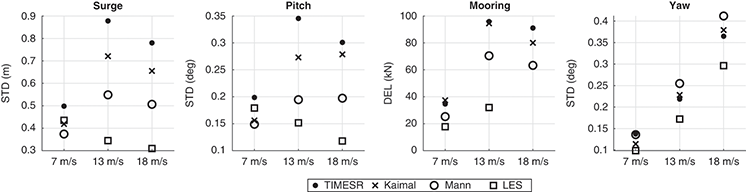
Figure 7.25 Standard deviation of the platform surge, pitch and yaw motion due to low frequency loads of the wind field only. For the mooring line loads a damage equivalent load (DEL) is given. Neutral atmospheric stability. 7, 13 and 18 m/s mean wind speed.
7.8 Control Issues for Floating Wind Turbines
7.8.1 Introduction
In discussing the control issues for bottom-fixed wind turbines (see Section 3.9), the main control objectives were to maximize power production below rated wind speed and to keep constant power above rated wind speed. It was also demonstrated that the controller should be designed with a slow response relative to the eigenfrequencies of the structure. The controller thereby reacts properly to variations in the incoming wind speed but does not interfere with the structural dynamics. An exception is when the controller is tuned to provide damping to, for example, the first fore-aft elastic bending mode of the tower.
For floaters, an additional perspective appears. Due to the rigid-body motions of the floater, the rotor may have a significant motion perpendicular to the rotor plane. The floater is also designed so that the rigid-body natural periods are outside the range of wave periods. This implies natural periods above 20 s for slack (catenary) moored floaters or below about 4 s for tension leg floaters. In this section the slack-moored floater is considered. The pitch natural period may be in the range of 25–50 s, while the surge natural period may be more than 1 min. When the rotor is moving toward the wind, the relative velocity between air and rotor increases. The control system, as outlined in Section 3.9, will interpret this as an increased wind velocity and as the period of motion period is so slow, the control system will adjust rotor speed, torque and blade pitch accordingly. As will be discussed, the effect may be a reduced or an increased damping of the floater motion. Other damping components such as wave radiation damping and viscous damping are low for such low-frequency motions. The floating wind turbine may thus require a modified control system to ensure proper damping and motion behavior.
7.8.2 Action of a Conventional Controller
Consider the turbine outlined in Figure 7.26. The wind is supposed to blow in positive
 -direction and the surge and platform pitch motions are considered only. The relative wind velocity at nacelle level can be written as:
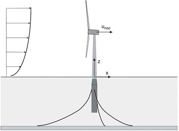
Figure 7.26 Coordinate system located at calm water level and velocity of horizontal nacelle motion.
 ([7.101])
Here,
 is the wind velocity at nacelle level and
 is the vertical position of the nacelle.
 and
and
 are the surge and pitch motions respectively. It is assumed that
 . It is further assumed that the motions are so slow that the control system adjusts the turbine to the stationary power and thrust. The thrust on the turbine is thus given by:
 ([7.102])
where
 is the rotor area and
 is the thrust coefficient.
To illustrate the effect of the rigid-body motion, one frequency of motion is considered only. This frequency may correspond to an eigenfrequency. As the eigenmode does not need to correspond to the modes as defined by the coordinate system, both a surge and pitch component need to be included. Each of the two velocity components are thus written as:

Here,
 is the phase of each component. During one cycle of oscillation the platform motion energy absorbed by the turbine may be written as:
 ([7.104])
Here
 .
.
7.8.2.1 Below Rated Wind Speed
Below rated wind speed, the controller is tuned for maximum power production. In this case both the power and thrust coefficients are almost constant.
 may thus be assumed to be constant in estimating the absorbed energy during one cycle of oscillation and [7.104] gives the following result:
 ([7.105])
Here,
 and
and
 is replaced by the mean wind velocity,
 . Using a linear 2DOF model, the damping force and dissipated energy over one cycle of oscillation can be written as:
 ([7.106])
Here,
 is the vector containing the (complex) surge and pitch velocities. Equating [7.105] and [7.106], the following elements in the damping matrix due to the rotor thrust are found:
 ([7.107])
 is in the order of 0.8–0.9 for wind velocities below rated. It is thus observed that the wind turbine contributes with a positive and, as can be shown, very significant damping when operating below rated wind speed and a conventional control system for bottom-fixed turbines is used. This is valid both for pitch and surge motions.
7.8.2.2 Above Rated Wind Speed
Above rated wind speed, the conventional blade pitch controller is set to maintain constant power and rotational speed. Thus, the thrust coefficient varies with the mean wind velocity, as demonstrated in Section 3.8. For the slow platform motions considered here, it may be assumed that the blade pitch controller and the thrust force behave almost as in the stationary case, i.e., there is no time delay between the change in relative velocity and corresponding thrust.
As a first approximation it is assumed that the thrust coefficient varies linearly with the relative wind velocity. This is an acceptable assumption for small velocity variations around the mean velocity
 . Thus, the thrust coefficient is written as:
 ([7.108])
Here,
 is the dynamic variation in the relative wind velocity due to the combined surge and pitch motion. It is assumed that
 . Under the above assumptions, the instantaneous thrust force becomes:

Let
 be harmonic with period
 and amplitude
 , then the absorbed energy, similarly as in [7.105], is obtained as:
 ([7.110])
The last term in the bracket may be disregarded as this is small (second-order) compared to the two other terms. Inserting for
 , the following expression is obtained for the energy absorbed during one cycle of oscillation:
 ([7.111])
This is the same expression as for the below-rated case, except for the last bracket. The linearized damping coefficients are thus obtained as:
 ([7.112])
Above rated wind speed, the slope of the thrust coefficient versus wind speed is negative.
 is thus negative. From [7.112] it is observed that the damping coefficients become negative if
 . In Figure 7.27,
 is plotted for the thrust characteristic of the NREL 5 MW reference turbine discussed in Section 3.8.1. It is observed that
 for velocities above rated wind speed.
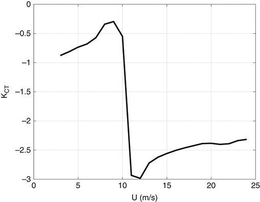
Figure 7.27
 as a function of mean wind velocity for the turbine with thrust curve as given in Figure 3.46. It is observed that
 for velocities above rated wind speed.
The consequences of this negative damping above rated wind speed have been illustrated both in numerical simulations and in full scale. Reference Skaare, Hanson, Yttervik and NielsenSkaare et al. (2011) demonstrated that a 2.3 MW turbine mounted on a spar foundation (the Hywind Demo turbine) exhibited negative damping for the platform pitch mode when operated with a conventional control system. Such behavior is also shown in simulations (see Figure 7.28).
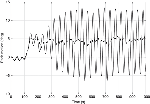
Figure 7.28 Platform pitch for a spar floating wind turbine. Tower pitch angle in degrees versus time. Mean wind speed 14 m/s and turbulent intensity 8.9%. Significant wave height 2.6 m, start-up from rest. Solid line: platform pitch with conventional turbine control; dashed line with motion controller switched on.
7.8.3 Control of Low-Frequency Motions
7.8.3.1 Controller for Bottom-Fixed Turbines
Reference Larsen and HansonLarsen and Hanson (2007) demonstrated by simulation the build-up of excessive motion of a floating wind turbine if a conventional controllerFootnote 2 was used above rated wind speed. They demonstrated how a bottom-fixed wind turbine with tower natural frequency of 0.5 Hz and a controller natural frequency of 0.1 Hz had a nice and stable response, while unstable behavior occurred after shifting the tower natural frequency to 0.05 Hz. Above rated wind speed they used a PI controller with constant torque and blade pitch control for rotor speed. The reason for using constant torque rather than constant power is to reduce dynamic loads in the drive train. The penalty is somewhat larger variations in output power.
To investigate further if the principles for the bottom-fixed turbine controller could be used for a floating wind turbine and obtain stable response, Reference Larsen and HansonLarsen and Hanson (2007) kept the PI controller and tested out four natural frequencies for the controller. The frequencies were 0.02, 0.04, 0.05 and 0.1 Hz. For each natural frequency they tuned the controller gains and studied the wind turbine behavior. The natural frequency of the turbine pitch motion was 0.035 Hz. From previous experience they aimed for a relative damping ratio of 0.8. They found that a controller natural frequency of 0.02 Hz was superior to the other choices, confirming the observations in Chapter 3 that the controller natural frequency should be significantly below the structural natural frequencies to avoid destructive interaction.
The controller proposed by Reference Larsen and HansonLarsen and Hanson (2007) removed the unstable behavior and reduced the platform pitch motion significantly. However, simulations in turbulent wind revealed large dynamic variations in quantities including power, torque and rotational speed. Increased variations in these quantities must be expected as the controller is too slow to adjust for the variation in the incident wind speed. Additional variations are to be expected when wave-induced motions are included.
The following section briefly discusses a couple of other options to avoid excitation of the modes with low natural frequencies, e.g., surge and pitch.
7.8.3.2 Use of a Notch Filter
A notch filter is a filter that is used to remove components of certain frequencies in a stochastic signal. A classic example is removing noise due to the 50 Hz grid frequency in electrical appliances. In the present case a notch filter is used to remove the input to the blade pitch control signal in a narrow frequency range. If this narrow frequency range is centered on the platform pitch natural frequency, the hypothesis is that the resonant excitation is avoided. Some basics about the notch filter and how it can be implemented in time domain are given in Appendix D. As shown in this appendix, a notch filter can be applied to a discrete stochastic time series
 to obtain a filtered time series
 by the following recursive function:
 ([7.113])
The coefficients
 and
and
 are obtained from the filter frequency, bandwidth and sampling interval.
The notch filter can be used in simulation models where the conventional controller is represented by, for example, a look-up table for the turbine thrust. The notch filter may then be used to simulate the floater motion controller. Used together with a conventional controller, problems may occur due to, e.g., the phase shift introduced by the notch filter. Assuming a linear relation between small variations in blade pitch angle and variation in thrust force, the effect of the notch filter will be illustrated by filtering the relative wind velocity between the wind and the turbine, governing the thrust force.
Transient Response Using a Notch Filter on the Wind Speed
Consider a spar-like floating wind turbine with 5 MW rated power. The main characteristics are given in Table 7.2.
| Dry Mass | Hydrodynamic Mass | |
|---|---|---|
| SurgeFootnote 3, M11 | 8149 Mg | 7797 Mg |
| Pitch, M55 | 6.377E7 Mgm2 | 3.800E7 Mgm2 |
| Coupled surge-pitch, M15 | -6.199E5 Mgm | -4.842E5 Mgm |
| Hydrostatic | Mooring | |
|---|---|---|
| Surge restoring, C11 | 47.070 kN/m | |
| Pitch restoring, C55 | 1123 MNm/rad | 239.600 MNm/rad |
| Coupled surge-pitch, C15 | -3.358 MN/rad |
The power and thrust coefficients for the turbine considered are shown in Figure 7.29. The coupled surge and pitch platform rigid-body motions are considered. A small linear damping (approximately 2%) is included in the model to account for an approximate hydrodynamic damping and to ensure stability of the numerical integration. The natural periods for the coupled surge-pitch system are obtained as 115.7 s and 29.8 s respectively. The longest natural period corresponds to an almost pure horizontal translation, while the fastest natural period corresponds to a rotational mode with center of rotation 69.1 m below the free surface, i.e., about midway between the center of buoyancy and the center of gravity.
The wind turbine is exposed to a wind field with mean wind speed 15 m/s at nacelle level and a turbulence intensity of 10%. The wind field is assumed to be coherent over the rotor disk area. A forward Euler integration scheme with time step 0.1 s is used for the simulations.
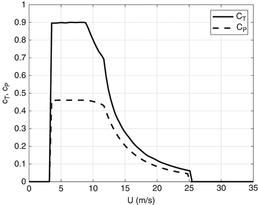
Figure 7.29 Power and thrust coefficients for the 5 MW turbine considered; see Table 7.2.

Two cases are considered in the simulations. First, a simulation is performed using the relative wind speed as input to the thrust force calculations and applying the quasi-static thrust characteristic to obtain the turbine thrust. The second simulation is performed in a similar way, the only difference being the relative wind speed, which now is passed through the notch filter prior to the thrust force calculation. The notch filter has a center frequency of 1/29.8 s, corresponding to the platform pitch natural frequency, and a bandwidth
 . The computed surge and pitch motions for the two cases are displayed in Figure 7.30.
From Figure 7.30 it is observed that initially the motions are dominated by the transient effects. This is to be expected as the initial position of the platform is at origin with zero platform pitch angle and the wind force is set on at full strength at t = 0. After a while the transient effects dies out. In the case without a notch filter, a large resonant pitch motion builds up. We have here an example of where the eigenmodes differ from the defined modes of motion. In the analysis, the pitch is defined as rotation about the y-axis, located at the water plane. However, the eigenmode for rotation has a center of rotation far below the water plane. Thus, the rotational eigenmode (“pitch mode”) also dominates the surge motion. The pitch motion is limited by the system damping and because excitation of the natural frequency is avoided by the use of the notch filter. Further, the relative wind speed drops below the rated wind speed during some of the oscillations. Below rated wind speed, the aerodynamic loads contribute to damping.
Applying the notch filter, the platform pitch motion dies out after the transient and has only small amplitude motions caused by the turbulent wind force. The surge motion shows some long periodic resonant motions. These is because the wind forcing at the surge natural period is not filtered out.
7.8.3.3 Motion Control Strategies
Section 3.9.3 discussed the control of a bottom-fixed wind turbine operation above rated wind speed. A PI control of the blade pitch angle was used:
 ([7.114])
where
 and
and
 are the proportional and integral gain respectively. If one considers a SDOF system, for example, the pure pitch motion of a floating wind turbine, it is possible to introduce a correction for the nacelle motion to avoid the negative damping discussed above. One may add a term proportional to the nacelle velocity on the right-hand side of [7.114],
 . This is a feedback term. Reference De SouzaDe Souza (2022) investigated this approach for a spar platform with a 20 MW wind turbine combined with a rotor torque control. De Souza found that the approach may have stability issues, in particular when introducing a low-pass filter on the input to the controller. The filter introduces a phase shift which reduces the stability.
To improve the stability of the above feedback control, a term proportional to the nacelle offset may be introduced. Then [7.114] is modified to:
 ([7.115])
Here,
 is a feed-forward gain, less than zero. Reference De SouzaDe Souza (2022) showed that this approached improved the stability even with a filter present.
Reference 376Skaare, Hanson and NielsenSkaare et al. (2007) used an estimator-based control strategy consisting of a numerical model of the wind turbine together with measurements to estimate the incoming wind. The measurements can be nacelle acceleration, thrust force rotor torque and/or power. Reference 376Skaare, Hanson and NielsenSkaare et al. (2007) implemented the estimator-based control system using a tool for computing the dynamics of floating wind turbines and found significant improved fatigue life of the tower due to the reduced pitch motion. A minor reduction in the mean power output was observed as well as some increased variability of power and rotational speed.
7.8.3.4 Use of Energy Shaping Control
Reference PedersenPedersen (2017) demonstrates how the negative damping can be mitigated by varying the rotor speed and thus using the rotor as an intermediate energy storage. He calls the principle “energy shaping control” (ESC). In the following, the main principle of the approach is outlined and demonstrated.
As above, the horizontal velocity of the floater at nacelle level is considered. Considering the combined surge and pitch motion, the velocity at nacelle level becomes
 .
.
It is assumed that the power output from the rotor follows the relative velocity between the wind and the rotor in a quasi-static manner, i.e., the delivered power from the rotor may be approximated by:
 ([7.116])
It is assumed that
 . At above-rated wind speeds, the conventional controller aims at keeping the power as well as the rotor speed constant. The thrust, and thus the power, is thus controlled by pitching the blades.
Now assume that the rotational speed of the rotor may vary. Ignoring losses, the equilibrium in instantaneous power may then be written as:
 ([7.117])
The first term in [7.117] is the power used for changing the kinetic energy in the rotor-generator assembly. Consider the variation around an equilibrium condition. At equilibrium
 ,
,
 and
and
 . I.e., for a small deviation from the equilibrium condition, [7.117] may be written as:

Now
 and
and
 . For small deviations from equilibrium, we thus obtain:
 ([7.119])
Omitting terms of higher order, and using [7.117], the following linear equation for the variation of the rotational speed is obtained:
 ([7.120])
Again, we observe that if the rotor velocity is constant,
 , the following relation is obtained:
 ([7.121])
That is, if the axial velocity of the rotor increases (in the direction of the incident wind) the thrust force also increases, and a negative damping effect is obtained.
To avoid this negative damping effect, Reference PedersenPedersen (2017) proposes allowing for variation in the rotational speed. The variation of the rotational speed is controlled by an augmented reference signal for the rotor speed controller. Pedersen thus assumes that the actual rotational speed
 is observed with high accuracy and that the set-point for the controller is augmented by a correction term
 such that the controller aims for a rotational speed of
 . The new rotational velocity is obtained by solving a differential equation with left-hand side equal to [7.120] but with a new right-hand side:
 ([7.122])
By requiring that the right-hand sides of [7.120] and [7.122] are equal, the following is obtained:

It is observed that for
 , the variation in thrust force will act in the opposite direction of
 , i.e., a positive damping is obtained. The thrust force on the turbine may now be written as:
 ([7.124])
Here,
 is the instantaneous incident wind velocity.
Now,
 ,
,
 is close to unity and
 is of order 1 but larger than 1. Thus, it is clear from [7.124] that the damping force is positive but small compared to the average wind thrust.
Use of Energy Shaping Control
The same 5 MW turbine as in the previous example is considered. The rotational inertia of the rotor-generator assembly is set to
 . The power is given by
 ,
,
 being the rotor torque. The derivative of the power with respect to the rotor velocity is obtained as:
 ([7.125])
For simplicity, it is assumed that the second term may be ignored. In lack of a proper controller, a perfect control of the rotational speed is assumed. I.e., the rotational speed obeys [7.122], where the nacelle velocity is obtained by solving for the combined platform pitch and surge motions. The instantaneous wind thrust is then obtained from [7.124]. Simulations with and without ESC are performed. In the ESC case the augmentation factor
 is set to 2.
First, a steady case with steady wind speed of 15 m/s is considered. The wind is started instantaneously at t = 0. In Figure 7.31 the computed surge and pitch responses are shown and compared for the two cases. A significant transient response is observed in both cases. In the initial phase the responses are similar for the case with and without ESC, but after a while the ESC case responses are attenuated and decay toward the steady-state value, about 15 m for surge and 3 deg for pitch. The case without ESC continues with large oscillations dominated by the pitch natural period. Figure 7.32 shows the corresponding variations in rotor thrust and rotational velocity.
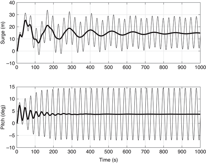
Figure 7.31 Steady 15 m/s wind. Initial surge and pitch = 0. Thick line: ESC with
 ; thin line: without ESC.

Figure 7.32 Variation in rotational speed and thrust for the ESC case in Figure 7.31.
Second, the same case as above is considered but including 10% turbulence intensity. A Kaimal wind spectrum is applied with coherence of 1 over the rotor area. The computed motions are shown in Figure 7.33. Large, almost steady-state pitch motions are obtained without the ESC, while in the ESC case the motions are reduced significantly after the end of the initial transient motions.
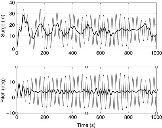
Figure 7.33 15 m/s mean wind with 10% turbulence intensity. Thick line: ESC with
 ; thin line: without ESC.
7.8.3.5 Examples from the Hywind Demo Development
In the development of the Hywind demo project, several new controllers were developed (see, e.g., Reference Nielsen, Hanson and SkaareNielsen, Hanson and Skaare, 2006; Reference Skaare, Hanson, Yttervik and NielsenSkaare et al., 2011; Reference 376Skaare, Hanson and NielsenSkaare, Hanson and Nielsen, 2007; and Skaare et al., 2014). The detailed specifications of the controllers are proprietary, but results from the implementation of two of them are given in Reference Skaare, Hanson, Yttervik and NielsenSkaare et al. (2011). The key idea is that the standard controller should work as before, keeping constant power production above rated wind speed and collectively adjusting the blade pitch angle to compensate for the variation in wind speed. The additional new motion controller “sits on top” of the standard controller, using the turbine motions as an extra input. By using the information of the turbine pitch motion an extra blade pitch signal can be given to provide the damping required to avoid excessive resonant motion, like what is demonstrated by the ESC in Section 7.8.3.4.
Similarly, as the blade pitch angle can be used to provide damping of the turbine pitch motion, one may use variation in generator torque to provide damping of the roll motion. In designing the controllers and determining the gains, one must evaluate issues such as: How much damping is needed? How do the motions influence fatigue of the structure? Does the controller impose excessive blade pitch activity and thus reduced lifetime of the actuators? Does the controller interact with nonresonant motions that are difficult to control, for example, wave-induced motions?
By a proper setting of the controller, energy from the wave-induced motions may be extracted by the wind turbine. This may have some relevance at below-rated wind speeds. The basic principles are given in Reference Nielsen, Hanson and SkaareNielsen, Hanson and Skaare (2006). The key challenge is that large motions will be required to extract a significant amount of energy.
7.8.4 Some Possible Dynamic Instabilities
7.8.4.1 Heave-Pitch (Roll) Coupling
Section 8.4 discusses the Mathieu instability in the context of a lifting operation from a moving crane. The vertical motion of the crane tip causes a variation in the tension in the lifting line. The line tension is entering into the restoring force for the pendulum motion of the load, and thus the equation of motion of the pendulum motion has a time-varying stiffness. The differential equation for the pendulum motion is an example of the Mathieu equation, which, in a more general form, may be written as:
 ([7.126])
Here, it has been assumed that the time variation in the stiffness term is harmonic.
 is the undamped natural frequency and
 is the damping ratio. It can be shown that the time-varying stiffness term may cause instability of the system. Even without any external excitation,
 may increase from an initial small value. For small
 , the instability occurs for
 . For larger
 , the range of instability increases, while increased damping reduces the range of instability (see Figure 8.8).
For a floating platform, pitch or roll motions may be excited by large heave motions. Consider the pitch motion of a spar substructure. The pitch-restoring term is given in [7.69] as:

Within linear theory,
 is a constant.Footnote 4 However, if the floating turbine performs large heave motions, and the pitch restoring is evaluated at the actual vertical position of the substructure, it is observed that both the displaced volume
 and the centers of buoyancy and gravity will vary with the heave motion (Reference Haslum and FaltinsenHaslum and Faltinsen, 1999). If the substructure has a heave motion
 , the change in submerged volume becomes
 , with
 being the water plane area of the substructure. The center of buoyancy will move
 upward. Thus, the pitch-restoring term in the heave-displaced position is obtained as:
 ([7.128])
For a spar substructure, the water plane area in most cases will contribute little to the pitch restoring. Thus, by accounting for the heave motion, the pitch restoring can be approximated by:
 ([7.129])
If
 is harmonic and
 in [7.126] is replaced with
 , the time-varying pitch-restoring term is obtained as:
 ([7.130])
Considering the regions of instability, large pitch (or roll) motions may occur if the ratio between the period of the heave motion
 and the pitch natural period
 is 1/2, 1, … . From Figure 8.8, it is observed that the range of instability is large in particular in the region around
 . Large heave motions may occur if the heave natural period is in the range of the wave periods. Therefore, a normal design requirement is for the heave natural period to be larger than the wave periods and the pitch natural period to be more than twice the wave periods.
For a lightly damped substructure, resonant heave motions may also be excited by second-order wave loads and other nonlinear effects. Reference Haslum and FaltinsenHaslum and Faltinsen (1999) demonstrate how a heave motion consisting of one component at a wave frequency and a slower component at the heave resonant period may contribute to Mathieu instability. The two motion components will create a heave envelope process with frequency
 . Thus, if the pitch natural frequency coincides with
 , large pitch motions may occur via the Mathieu instability. The nonlinear effect causing heave at the heave natural period is a coupling effect between the heave and pitch motion. When the spar substructure performs a pitch motion, forces acting perpendicular to the axis of the spar cause a vertical force. The heave motion at resonance is thereby amplified, which, via the Mathieu instability, again amplifies the pitch motion. Increased heave and pitch damping will mitigate the resonant responses.
7.8.4.2 Roll-Yaw Coupling
Reference Haslum, Marley, Navalkar, Skaare, Maljaars and AndersenHaslum et al. (2022) point out an aerodynamic coupling effect that may cause large roll and yaw motions of a floating wind turbine. They illustrate the effect by considering a spar platform. The effect may be explained as follows. Consider a spar substructure, as illustrated in Figure 7.1. However, to minimize the coupling effects in the inertia matrix, the origin of the coordinate system is moved downward to the CG of the floating turbine. For simplicity only the roll and yaw motions are considered. Under the assumption that the thrust
 on the rotor acts perpendicular to the rotor plane, the thrust in
 and
and
 -direction becomes
 and
and
 . The thrust acts a distance
 above origin, thus the roll and yaw moments due to the thrust may be written as:
 ([7.131])
Here, small rotations have been assumed and the aerodynamic stiffness coupling terms
 introduced. Assuming a diagonal mass matrix and that the linearized hydrostatic and mooring stiffnesses are also diagonal, the inertia and stiffness matrices for the coupled roll-yaw motion may be written as:
 ([7.132])
The eigenvalues for the undamped system are obtained using [5.21]:
 ([7.133])
Without the last term, representing the aerodynamic coupling, the two solutions for
 represent the two uncoupled natural frequencies,
 ,
,
 . Including the coupling term, but with a weak coupling so the term inside the square root sign still is positive, two real natural frequencies are still obtained. If the coupling term increases so that the term inside the square root becomes negative, the natural frequencies become complex, i.e.,
 . Thus, the undamped response will behave as:
 ([7.134])
The first term represents a harmonic oscillation while the second term represents an exponential decaying term and an exponential growing term. Thus, to avoid instability in the undamped case, the term under the square root sign in [7.133] must be positive. This can be expressed as a requirement to the frequency difference between the uncoupled roll and yaw frequencies:
 ([7.135])
As
 , the requirement to the difference between the roll and yaw natural frequencies increases as the thrust force increases and as the distance between the CG and the nacelle increases.
The above considerations illustrate the main causes of the instability of the coupled roll-yaw motion. Reference Haslum, Marley, Navalkar, Skaare, Maljaars and AndersenHaslum et al. (2022) have studied the phenomenon using a state-of-the-art computer program for floating wind turbines. Due to several coupling effects, nonlinearities and damping, an exponential increase of the motions is not observed, but rather limit-cycle motion responses. An important observation is that damping may reduce the limiting thrust force for stability as given by [7.135]. This is explained by the fact that a phase shift between the two motions will cause the thrust force to partly act in phase with the motion velocity. Damping causes such a phase shift. A force acting in phase with the motion velocity will transfer or extract energy into that mode of motion.
Exercises Chapter 7
1. Write down the (linear) contribution to the 6DOF restoring matrix for a tension leg platform with four vertical tethers in a quadratic pattern. Define the quantities involved.
2. Write down the (linear) contribution to the 6DOF restoring matrix from a tension leg platform with three vertical tethers in symmetric triangular pattern. Define the quantities involved.
3. Consider a four-legged tension leg platform with a quadratic layout and consider loads in the
-direction only (see Figure 4.7).
a. Use quasistatic considerations and derive the relation between the wind thrust at nacelle level and the tether loads.
b. Find a criterion for the minimum pretension in the tethers to avoid slack.
c. Make a similar consideration as in Exercises 3a and 3b, but assume the loads are wave loads acting at the water line level.
4. The stiffness of a catenary mooring line consists of an elastic and a geometric contribution. Show how the total stiffness is obtained by combining the two.
5. Assume a wind turbine tower can be modeled as a vertical beam with uniform mass distribution. The tower is 120 m tall and has a mass of 5000 kg/m. Compute the 6DOF mass matrix for the tower when:
a. the center of the coordinate system is at the bottom of the tower and the z-axis coincides with the tower axis.
b. the center of the coordinate system is at the bottom of the tower and the z-axis is displaced 20 m in the negative
-direction and 10 m in the negative y-direction. The z-axis is parallel to the tower axis.c. the tower is located as in Exercise 5b and a nacelle modeled as a point mass of 450 Mg is located on top of the tower.
6. Consider the vertical wave forces on a spar platform (see Figure 7.7). The diameter of the lower part is
and of the upper part is
. The lower part of the cone starts at draft
and ends at
. The draft of the spar is
.
a At which draft will you replace the cone with an abrupt change in diameter?
b Assume deep-water waves. At which wave frequency will we have zero vertical wave force? Assume you may estimate the wave force by the Froude-Krylov contribution.
c Write down the expression for the heave natural frequency.
7. Consider a semisubmersible as outlined in Figure 7.10. We will consider the two columns and the single pontoon only. The waves are assumed to propagate in the direction of the pontoon axis. The pontoon is 30 m long, 5 m wide and 3 m high. The bottom of the pontoon is located 20 m below the water surface. The columns have a square cross-section with the length of each side equal to 5 m. Deep-water waves may be assumed.
a. For which wave period do we obtain cancellation of the heave wave force? Use the Froude-Krylov approximation.
b. For which periods do we expect cancellation of the wave forces in surge?
c. For which wave period do we obtain cancellation of wave forces in pitch? Use the Froude-Krylov approximation and make an estimate both by ignoring and including the horizontal forces of the columns.
8. In [7.63] the drag force on an element is given by considering the relative motion between the fluid and the motion. Assume a sinusoidal motion velocity of both fluid and body. Consider four different phases between the motion velocity and the fluid velocity, 0,
,
and
, and assume the amplitude of the fluid velocity to be twice the body velocity.
a. What is the minimum and maximum drag force on the body during one cycle of oscillation in the four cases?
b. What is the dissipated damping energy during one period of oscillation in the four cases?
9. Assume a synthetic mooring line has a diameter of 0.12 m and a minimum breaking strength (MBS) of 10 MN. Assume that the mean tension in the line is 20% of the MBS. How large is the difference between the effective tension and the real tension in the line as a function of water depth?
10. Consider the thrust coefficient displayed in Figure 7.29 and consider a floating wind turbine with the nacelle 120 m above sea level and a natural period in pitch of 30 s. Consider platform pitch only. The static platform pitch at 7 m/s wind speed is 2 deg. Ignore damping and make a SDOF simulation routine and consider the following cases.
a. Start with an initial platform pitch angle of 2 deg and use a steady wind speed of 7 m/s, 10 m/s, 12 m/s and 20 m/s (you may use
from Figure 7.27.) Discuss the motion behavior in the various cases.b. Use one of the wind time histories in “WindTimeSeries.txt” and scale the velocities so that mean wind speeds of 7 m/s, 10 m/s, 12 m/s and 20 m/s are obtained. Check if the obtained turbulence level is reasonable. Simulate the dynamic response.
11. Show how the linear dynamic equation for the rotational speed in [7.120] is obtained.
12. Consider a spar-like floating wind turbine with the following main particulars. The substructure has only one diameter. Assume the vertical mass distribution of the tower and substructure to be uniform. Three mooring lines are used, placed symmetrically around the substructure. Main data is as follows.


from z = 0 to z = −95 m −39 m from −95 to −79 m −87 m Horizontal stiffness single mooring line: Vertical stiffness single mooring line: −20 mHeight of rotor center: 70 m Rotor diameter: 82 m Thrust coefficient: 0.8 Wind speed: 10 m/s Tower: from z = 0 to z = 68 m Substructure: RNA mass: 140 Mg Center of gravity RNA,
 :
:70 m Tower mass: 170 Mg Center of gravity tower,
:32 m Substructure mass: 1300 Mg Center of gravity substructure,
:Radius substructure: 4.1 m Ballast: Center of gravity ballast,
:18 kN/m 2 kN/m Vertical connection of mooring lines:
Consider the surge, heave and pitch motions only. The origin of the coordinate system is at the water line level. Compute:
a. mass of ballast (ignore the vertical load from the mooring and power cable)
b. mass matrix
c. added mass matrix
d. hydrostatic restoring matrix
e. mooring line restoring matrix
f. natural frequencies with and without mooring attached
g. static pitch due to wind thrust
h. wave excited motions in surge, pitch and heave due to a wave with an amplitude of 1 m propagating in positive x-direction. Use strip theory. Use a range of wave periods from 3 to 40 s. Assume infinite water depth
13. Show how the linearized damping in [7.39] is obtained.


