


1 Introduction
Given that formal insurance markets in developing countries are very limited, poor households typically rely on the help of family or friends in times of economic hardship. These informal exchanges of gifts, loans or labour, which are motivated by social preferences or strategic incentives, serve de facto as risk pooling devices and are an important, though incomplete source for households to cope with negative income shocks.Footnote 1 A large body of literature investigated forms, motives and constraints of such informal risk-sharing arrangements (see Fafchamps Reference Fafchamps, Benhabib, Bisin and Jackson2011). A much smaller literature studies the relationship between mutual support and the extent to which individuals can control their risk exposure. A growing body of evidence suggests that a considerable proportion of individuals favour redistribution when inequalities are caused by exogenous circumstances rather than by factors of personal responsibility (e.g. Schokkaert and Devooght Reference Schokkaert and Devooght2003; Krawczyk Reference Krawczyk2010; Le Clainche and Wittwer Reference Le Clainche and Wittwer2015; Roemer and Trannoy Reference Roemer, Trannoy, Atkinson and Bourguignon2015).
Existing evidence on the question whether the extent to which individuals can control their risk exposure affects the willingness to share income is coming from two strands of literature. The first one comprises experimental studies conducted in high-income Western countries. Bolle and Costard (Reference Bolle and Costard2015) and Cappelen et al. (Reference Cappelen, Konow, Sorensen and Tungodden2013) study fairness views towards risk-taking and find that subjects who favour redistribution ex post make a distinction between inequalities that result from differences due to luck and due to deliberate choices. Trhal and Radermacher (Reference Trhal and Radermacher2009), Cettolin and Tausch (Reference Cettolin, Riedl and Tran2015) and Akbas et al. (Reference Akbas, Ariely and Yuksel2019) contrast the situation where subjects are exposed to exogenous income risk with the situation where subjects can choose freely between a risky and a safe(r) income option. They find supporting evidence for the hypothesis that individuals are less generous towards those whose bad outcome is a result of their own risk-taking action compared to just bad luck. Yet, these findings are not necessarily transferable to developing countries, which are the focus of our study. The countries in which the studies have been conducted have social security systems that considerably limit the extent to which individuals need to rely on other people’s solidarity. Such public safety nets are absent in developing countries and mutual voluntary help is an essential risk-pooling source for households. This is supported, for example, by Jakiela (Reference Jakiela2015), who finds that Kenyan villagers make virtually no difference in their allocation decisions with respect to whether income was earned by exerting real effort or the result of pure luck, while the contrary was the case for US students. Schokkaert and Devooght (Reference Schokkaert and Devooght2003) compare students in Belgium, Burkina Faso and Indonesia regarding answers to hypothetical questions about the fair distribution of ex post tax income and subsidies for health expenditures. When participants think that individuals are responsible for their behaviour (e.g. through smoking or low effort), the degree to which subjects favour no compensation or punishment of the responsible person differs strongly by country, pointing to relevant differences in fairness perceptions.
The second strand of literature is a series of experimental studies that investigate whether the introduction of voluntary formal insurance in developing countries has a crowding-out effect on informal mutual support (Landmann et al. Reference Landmann, Vollan and Froelich2012; Lin et al. Reference Lin, Liu and Meng2014; Anderberg and Morsink Reference Amendah, Buigut and Mohamed2020; Lenel and Steiner Reference Lenel and Steiner2020) which is supported by their findings.Footnote 2 The experimental designs have in common that they exogenously expose participants to a risky outcome in one treatment, and allow them to reduce this level of risk exposure by choosing an insurance option in a second treatment. By doing so, these studies deal with a special case of risk avoidance, though. Insurance is a device to opt out of risk, while we are interested in more general situations that include opting into risk. The latter is particularly important in developing countries, which are characterized by underinvestment in profitable business opportunities, leaving much of the earnings and growth potential unexploited (De Mel et al. Reference D’Exelle and Verschoor2008; McKenzie and Woodruff Reference McKenzie and Woodruff2008; Grimm et al. Reference Grimm, Knorringa and Lay2011, Reference Grimm, Kruger and Lay2012; Banerjee and Duflo Reference Banerjee and Duflo2014; Fafchamps et al. Reference Fafchamps, McKenzie, Quinn and Woodruff2014; Dodlova et al. Reference Dodlova, Göbel, Grimm and Lay2015; Kremer et al. Reference Kremer, Lee, Robinson and Rostapshova2016).Footnote 3 We argue that fairness views with respect to risk avoidance might differ from those regarding risk taking. Opting into a risky income opportunity involves the chance to earn a high income that may also benefit risk-sharing partners. This might be considered as more acceptable than foregoing precautionary actions, such as insurance take-up, which would preserve the status-quo-income against losses. With this more general view on risk taking, our paper is also related to the literature on risk sharing and investment behaviour in developing countries (see, for example, D’Exelle and Verschoor (Reference De Mel, McKenzie and Woodruff2015) and the literature reviewed in this paper). Moreover, we avoid the caveat of the insurance literature that the validity of the measured impact on solidarity critically hinges on a proper understanding of, and some familiarity with the concept of insurance, which is typically not given for the majority of people in less developed countries (cf. Lenel and Steiner Reference Lenel and Steiner2020).
Therefore, as a first contribution, we adapt the more general experimental settings used for studying the relationship between risk taking and income sharing in Western countries to the context of a developing country. We conducted a laboratory experiment with slum dwellers in Nairobi, Kenya. In a between-subject design with two randomized treatments similar to Cettolin and Tausch (Reference Cettolin, Riedl and Tran2015), each participant could either choose (treatment CHOICE) or was randomly assigned (treatment RANDOM) to a project with either a safe or a risky income. The risky option involved a one-half probability to end up with nothing, and we framed it as an investment opportunity in order to emphasize the perspective of opting into risk. After being randomly and anonymously matched with another person in the same treatment, subjects could make voluntary transfers to their partner. We elicit transfers for all possible choices and situations of the partner independent of the realized states. This rules out strategic interactions and allows us to conduct comparisons of transfers to partners who chose different projects in addition to the comparisons across treatments, which is informative about the mechanisms behind reduced solidarity.
The second contribution is a methodological one. We are the first to show that in experimental settings where potential donors make the decision about transfers rather than uninvolved outsiders, such as the ones used in Trhal and Radermacher (Reference Trhal and Radermacher2009), Cettolin and Tausch (Reference Cettolin, Riedl and Tran2015) and Akbas et al. (Reference Akbas, Ariely and Yuksel2019),Footnote 4 the comparison of mean transfers across treatments does not isolate the main behavioural effect of interest. This comparison is confounded by the fact that randomization to projects in RANDOM unavoidably creates a group of subjects for which there are no comparisons in the CHOICE treatment, namely subjects that are assigned to a project that they would not choose for themselves. If this group exhibits different transfers than the group assigned to their preferred project, then transfers could differ across treatments for other reasons than different fairness views. For example, donors in RANDOM may compensate themselves for the utility loss associated with being in an unwanted project by giving less to others. Moreover, Cettolin and Riedl (Reference Cettolin and Riedl2017) and Cettolin et al. (Reference Cettolin and Tausch2017) find that other-regarding preference depend on risk preferences. To identify the subjects in RANDOM, for whom assigned and preferred project differ, we use an experimental design that elicits preferred projects for all subjects in RANDOM.Footnote 5 This allows us to compare subjects across treatments that prefer the same project, which enables us to isolate the behavioural effect of CHOICE we are interested in.
Another advantage of this design is that it enables us to compare the effect of CHOICE for different combinations of donor’s and partner’s project. This, in turn, allows us to discriminate between different possible explanations for reduced transfers in CHOICE, which is the third contribution of our paper. Without the ability to align project preferences across treatments, comparing transfers of subjects with the same project across treatments is flawed by selection bias that results from the fact that subjects who chose a given project in CHOICE systematically differ from the subjects randomly assigned to the same project in RANDOM. The first possible explanation for reduced transfers is attribution of responsibility for neediness when partners self-select into the risky project that is motivated by a shared norm about low risk-taking. Here we exploit that only transfers to partners choosing the risky project should fall but not those to partners choosing the safe project, if attributions of responsibility are the driver behind reduced transfers. The second possible explanation is a form of what one could call ex-ante choice egalitarianism. Donors who deliberately choose an option that results in higher income may be less willing to share their high payoff compared to receiving the same payoff by pure luck, because subjects have the same ex-ante opportunities for choosing a specific option. If this is the case, then we should observe that donors make lower transfers in CHOICE independent of the partner’s choice of project. Another possibility is ex-post choice egalitarianism as discussed by Cappelen et al. (Reference Cappelen, Konow, Sorensen and Tungodden2013), where subjects view income inequalities as fair if they result from different choices but as unfair if they are due to different outcome realizations that result from the same choice. In this case, transfers should only be lower when donor’s and partner’s choice of project differ but not when they are the same.
With our design we find that free choice of risk exposure reduces transfers but only for donors who themselves prefer the risky project. Moreover, this reduction is independent of the partner’s choice of project. As a result, we reject both attributions of responsibility for neediness, and ex-post choice egalitarianism as possible explanations for reduced transfers. Instead, we find that risk-takers seem to feel less obliged to share high payoffs that result from their choices compared to the situation where high payoffs are the result of pure luck. This suggests that a substantial share of subjects have fairness views that are in line with ex-ante choice egalitarianism, which emphasizes the fact that everybody had the chance to pick the risky project and be lucky in CHOICE but not in RANDOM. We also find that risk choosers seem to take responsibility for their own risky choice by expecting less from others in case they end up with nothing. These findings are in line with D’Exelle and Verschoor (Reference De Mel, McKenzie and Woodruff2015), who study investment behavior and risk sharing in a lab-in-the-field experiment in Uganda and find that investors in risky opportunities share less of both their profits, and their losses.
Overall it seems that the strong norm of mutual support in developing countries works against severe punishment of risky choices and makes risk choosers aware of the burden their investment behavior may impose on others. In this respect, our findings differ substantially from the evidence for Western countries. Moreover, the fact that our results also differ from the evidence on crowding out of informal insurance by the availability of formal insurance for developing countries, suggests that fairness views regarding risk avoidance may differ from those regarding opting into risk with the potential of realizing higher payoffs that may benefit risk-sharing partners. Thus, our results suggest that not only the social norm regarding solidarity in a society matters, but also the situation in which individuals make choices that involve risk (opting into or out of risk). Our findings have important implications for policies that aim to encourage entrepreneurship or investments into new but risky business opportunities to reduce poverty and foster economic growth in developing countries.
The remainder of the paper is organized as follows. The next section describes the experiment we conducted in detail. In Section 3 we derive the hypotheses for the empirical analysis. Here we explain in detail how our experimental design allows isolating the behavioural effect of interest and discriminating between different explanations. Section 4 addresses potential concerns about our experimental design. In Section 5 we present and discuss our results. The last section concludes. An appendix contains supplementary information and material.
2 The experiment
2.1 Experimental context
We conducted a laboratory experiment at the Busara Center of Behavioral Economics in Nairobi, Kenya. The centre provides a state-of-the-art lab infrastructure, including up to 25 computer-supported workplaces. It maintains a subject pool with currently around 12,000 registered individuals, many of them recruited from the Nairobi informal settlement Kibera. The living situation in this slum community is characterized by extreme poverty and insecurity due to the lack of property rights and high criminality. Housing and hygiene conditions are very poor since the government does not provide water, electricity, sanitation systems or other infrastructure (The Economist Reference Economist2012). Most of the slum residents work as small-scale entrepreneurs and casual workers in the informal sector, therefore relying on uncertain and irregular income streams. Related to the lack of formal employment, most of the slum dwellers have no formal risk protection such as health insurance (Kimani et al. Reference Kimani, Ettarh, Kyobutungi, Mberu and Muindi2012). Many households are, however, member in some kind of social network, such as merry-go-rounds, which allow saving and borrowing and implicitly provide an informal safety net (Amendah et al. Reference Amendah, Buigut and Mohamed2014).
In Kenya, in general, there is a strong spirit of harambee (the Swahili term for ’pulling together’) which encloses ideas of mutual support, self-help and cooperative effort. Harambee takes various forms, such as local fundraising activities to help persons in need or the joint implementation of community projects (e.g. building schools or health centers). While being an indigenous tradition in many Kenyan communities, the concept became a national movement since Kenya’s first president Komo Kenyatta used it as slogan for mobilizing local participation in the country’s development (Ngau Reference Ngau1987; Mathauer et al. Reference Mathauer, Schmidt and Wenyaa2008; Jakiela and Ozier Reference Jakiela and Ozier2016). In the light of this strong tradition of solidarity and seemingly well-established informal security nets it is therefore particular interesting and important to understand which behavioural mechanisms drive willingness to support others.
2.2 Experimental design
2.2.1 Risk solidarity game
The core game of the study aims at measuring solidarity behaviour in situations where subjects either can choose or are exogenously assigned to a certain risk exposure. Figure 1 gives an overview on the sequence of steps in the game. At the beginning, two projects were presented to each subject: a safe option offering 500 KSh and a risky alternative yielding either 1000 or 0 KSh with equal probability. Depending on the treatment, subjects could either choose (treatment CHOICE) or were randomly assigned with probability 0.5 (treatment RANDOM) to one of these two options (step 1). After having chosen one project or being informed about the randomly received option, each subject was randomly and anonymously paired with another person in the room, who followed the same experimental procedure and was hence in the same treatment condition as the subject herself (step 2).Footnote 6

Fig. 1 Sequence of steps in the risk solidarity game
Before informing the subjects about their own realized payoff and their matched partner’s project and earnings, we elicited their conditional transfers using the strategy method (step 3). Thereby, all subjects were asked how much of their project income they wanted to transfer to the partner if the partner earned (1) 500 KSh from the safe project, (2) 1000 KSh from the risky project, or (3) 0 KSh from the risky project. Subjects with the safe project made these three transfer decisions based on their sure income of 500 KSh, while subjects with the risky project stated their three gifts in case of winning the high project payoff of 1000 KSh. Risky project holders could not make any transfer in case of earning the zero payoff of their option. Although we are interested in solidarity from better-off to worse-off persons and will exclusively evaluate these transfers in the following analyses, we nevertheless elicited transfers for all three possible payoffs of the partner (including situations where the partner is equally well or better off than the donor) in order to keep the decision task neutral and symmetric across project holders.
After the transfer statements, subjects were asked in a similar way which monetary amount they expected to receive from their partner if the partner earned (1) 500 KSh from the safe option, or (2) 1000 KSh from the risky option (step 4). Subjects with the safe project stated their expectations based on their sure earnings of 500 KSh, and subjects in the risky option stated their beliefs in case of winning zero shillings, respectively.Footnote 7 At the end of the experiment, the lottery outcomes of all participants were individually determined (step 5). Subjects had been informed at the beginning of the game that their own and the partner’s payoffs would be established by two different random draws. Transfers between the partners were then effected according to the actually realizing states. The stakes of the game represented considerable amounts for the mainly very poor participants who reported an average daily income of 160 KSh (
 1.50 USD).
The design implies that in the RANDOM treatment, subject’s income is determined purely by chance, while in the other treatment, it can be influenced by the participant’s choice. In particular, becoming a needy person, i.e. earning the zero income from the lottery, is just bad luck in RANDOM but involves a voluntary decision for the risky lottery in CHOICE. The imposed trade-off between a safe and a risky option thereby ensures that risk taking is salient to the participants. Moreover, since the payoffs of the two alternatives both equal 500 KSh in expectation, the risky option reflects a mean-preserving spread of the safe alternative implying that taking the risk is not compensated by higher expected income. Hence, choosing the lottery is not utility maximizing for risk averse individuals and possibly unnecessary in the risk-sharing partner’s view since avoiding the risk is not costly. This case has also been studied in the related experimental literature (e.g. Trhal and Radermacher Reference Trhal and Radermacher2009; Bolle and Costard Reference Bolle and Costard2015; Cettolin and Tausch Reference Cettolin, Riedl and Tran2015). It provides an important benchmark for the effect of risk exposure choice on solidarity in alternative scenarios in which risk taking is either beneficial or even unfavorable in terms of expected income. Moreover, it allows us to distinguish subjects with distinct risk preferences (risk averse or not) without having to make assumptions about the underlying utility function.
The design as an anonymous one-shot game deviates from conditions of real-world solidarity in developing countries, which typically takes place among persons within the family or neighbourhood in repeated exchanges. Keeping subjects’ identity confidential is, however, necessary in order to avoid that possible real-life relationships or fear of sanctions outside the lab bias behaviour of participants. Further, by restricting the game to one single round we implicitly rule out that subjects base their risk-taking and sharing decisions on strategic considerations induced by repeated interactions. This isolates the effect of risk taking on giving behaviour motivated by (social) preferences, such as altruism or distributive preferences (cf. Charness and Genicot Reference Charness and Genicot2009). It represents an important reference case since it avoids that possibly interacting intrinsic and extrinsic motivations blur the measured impact. Overall, since our design excludes issues of social pressure and reciprocity considerations that probably would have reduced the participants’ incentives to punish a risk-taking partner, our experiment is likely to measure an upper bound of the behavioural effect of risky choices on solidarity.
2.2.2 Elicitation of project preferences
In the CHOICE treatment, subjects reveal their project preference by the choice they make in step 1 of the game (see Fig. 1). In the RANDOM treatment, we elicit subjects’ preferred project after subjects have made their statements about own and expected transfers but before realization of outcomes, i.e. between steps 4 and 5 in Fig. 1. At this point, we asked subjects which of the two projects they would have chosen had they had the possibility to do so.Footnote 8 We did not inform subjects ex ante that this question would come up to ensure that all steps of the game before this question are unaffected. Eliciting preferences before realization of outcomes rules out that considerations such as regret affect preference statements. Doing so after transfer statements in steps 3 and 4 of the game ensures that stated transfers are unaffected by preference elicitation. An alternative approach, which has been used in other contexts,Footnote 9 is to let subjects select their preferred option and then a randomization device determines whether choices are actually implemented. However, Long et al. (Reference Long, Little and Lin2008) and Marcus et al. (Reference Marcus, Stuart, Wang, Shadish and Steiner2012) show that denying subjects their preferred choice can affect behaviour (in our case stated transfers in RANDOM) and, thus, confound the effects we are interested in.
Furthermore, we did not incentivize this question, i.e. we did not make payoffs dependent on the preference question in RANDOM. Since we inform subjects before the game how their final payoff will be determined, we would have had to reveal that the question about project preference will come up. Again, this bears the risk of affecting transfer statements, which we wanted to avoid. The fact that there are no incentives to answer truthfully, naturally raises the question whether we measure project preferences in RANDOM correctly. To address this concern, we added an auxiliary treatment with a third subject pool. The sole task in this incentivized game was to choose between the safe and risky project as in step 1 of the CHOICE treatment. However, the participants played this game in full autarky, i.e. they were not paired with another individual and transfers were not possible. The payoffs of this game corresponded to the safe amount or the realizing lottery outcomes, respectively. With the auxiliary experiment we can assess whether real monetary consequences matter for stated preferences by comparing the choices made in this experiment to the non-incentivized preference statements in the RANDOM treatment. Furthermore, we can address the issue that in the CHOICE treatment, subjects’ decisions on projects might be driven strategically by subsequent transfer decisions. The subjects in CHOICE knew that they would have to decide on transfers after their choice of project. This could affect their decision because the probability to face a partner who is worse off differs by project. If this was the case, then chosen projects in CHOICE would not reflect project preferences. Yet, if we find no differences in choices and stated preferences both in the main experiment between CHOICE and RANDOM, and between the main and auxiliary experiment, then this supports the validity of our experimental design with respect to both concerns. We discuss this in detail in Sect. 4.2.
2.2.3 Procedures
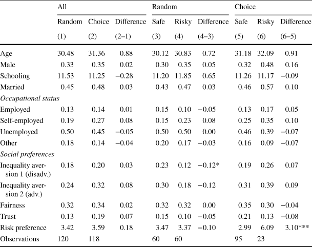
For recruitment, subjects were randomly chosen from the Kibera subject pool registered at Busara and then invited by SMS. A precondition for being selected was an education level of at least primary school (8 years) to ensure some familiarity with numerical values as is necessary for our study. Using a between-subject design, the recruited persons were randomly assigned to one of the two treatments. The core experiment was run within 13 sessions in December 2017. Six sessions were conducted of the RANDOM treatment and seven of the CHOICE treatment. As a result, all subjects in the same session are also in the same treatment.Footnote 10 Moreover, subjects in a given treatment were not aware of the existence of the other treatment. Hence, we can rule out that within-session dynamics explain differences across treatments. In total, 238 subjects participated in our study, thereof 120 in RANDOM and 118 in CHOICE. 33% of our subjects are male and 47% are married. On average, the participants are 31 years old and have a schooling level of 11 years. Table 1 gives an overview on selected basic characteristics of the participants by treatment and project. In addition, we ran 5 sessions of the auxiliary treatment in January 2018 where, in total, 111 subjects participated.
Table 1 Basic characteristics of participants by treatment and project
|
All |
Random |
Choice |
|||||||
|---|---|---|---|---|---|---|---|---|---|
|
Random |
Choice |
Difference |
Safe |
Risky |
Difference |
Safe |
Risky |
Difference |
|
|
(1) |
(2) |
(2–1) |
(3) |
(4) |
(4–3) |
(5) |
(6) |
(6–5) |
|
|
Age |
30.48 |
31.36 |
0.88 |
30.12 |
30.83 |
0.72 |
31.18 |
32.09 |
0.91 |
|
Male |
0.33 |
0.35 |
0.02 |
0.30 |
0.35 |
0.05 |
0.32 |
0.48 |
0.16 |
|
Schooling |
11.53 |
11.25 |
−0.28 |
11.20 |
11.85 |
0.65 |
11.26 |
11.17 |
−0.09 |
|
Married |
0.45 |
0.48 |
0.03 |
0.43 |
0.47 |
0.03 |
0.46 |
0.57 |
0.10 |
|
Occupational status |
|||||||||
|
Employed |
0.13 |
0.14 |
0.01 |
0.15 |
0.10 |
−0.05 |
0.13 |
0.17 |
0.05 |
|
Self-employed |
0.19 |
0.27 |
0.08 |
0.15 |
0.23 |
0.08 |
0.25 |
0.35 |
0.10 |
|
Unemployed |
0.50 |
0.45 |
−0.05 |
0.50 |
0.50 |
0.00 |
0.46 |
0.39 |
−0.07 |
|
Other |
0.18 |
0.14 |
−0.04 |
0.20 |
0.17 |
−0.03 |
0.16 |
0.09 |
−0.07 |
|
Social preferences |
|||||||||
|
Inequality aversion 1 (disadv.) |
0.18 |
0.20 |
0.03 |
0.23 |
0.12 |
−0.12* |
0.19 |
0.26 |
0.07 |
|
Inequality aversion 2 (adv.) |
0.24 |
0.32 |
0.08 |
0.30 |
0.18 |
−0.12 |
0.31 |
0.39 |
0.09 |
|
Fairness |
0.32 |
0.34 |
0.02 |
0.32 |
0.32 |
0.00 |
0.35 |
0.30 |
−0.04 |
|
Trust |
0.13 |
0.19 |
0.07 |
0.15 |
0.10 |
−0.05 |
0.21 |
0.13 |
−0.08 |
|
Risk preference |
3.42 |
3.59 |
0.18 |
3.47 |
3.37 |
−0.10 |
2.99 |
6.09 |
3.10*** |
|
Observations |
120 |
118 |
60 |
60 |
95 |
23 |
|||
*, **, *** indicates significance on the 10/5/1% level
Upon arrival, subjects were identified by fingerprint and randomly assigned to a computer station. The instructions were then read out in Swahili by a research assistant, while simultaneously, some corresponding illustrations and screenshots were displayed on the computer screens (see online Appendix F for an English version of the instructions, exemplarily for CHOICE).Footnote 11 For the entire experiment the z-Tree software code (Fischbacher Reference Fischbacher2007) was programmed to enable an operation per touchscreen which eases the use for subjects with limited literacy or computer experience. Subsequently, some test questions verified the participants’ comprehension of the game rules. In case of a wrong answer, the subject was blocked to proceed to the following question. A research assistant then unlocked the program and gave some clarifying explanations if needed. This procedure aimed at increasing the likelihood that all participants fully understood the games. After the comprehension test, the participants performed the actual experimental task. The experiment involved, firstly, a risk preference game which aimed at measuring subjects risk attitudes (see online Appendix E for details) and, secondly, the risk solidarity game explained in detail in the previous section.Footnote 12 Importantly, the subjects completed the decisions in these two games without learning the realized payoff in the precedent game. Moreover, after randomly determining the game payoffs at the end of the experiment, only the result of one randomly selected game was relevant for real payment. These two design features avoid that results are biased due to any strategic behaviour, expectation forming or income effects across games.
At the end of the session, participants completed a questionnaire covering important individual and household characteristics. After the session, subjects received 200 KSh in cash as show-up fee which compensated mainly for the travel costs to the center. Moreover, subjects earned a minimum of 250 KSh in the experiment in order to guarantee an appropriate compensation for the time spent. However, participants were not informed about this minimum compensation before the end of the game. In total, average earnings amounted to 447 KSh per person. They were transferred cashless to the respondents’ MPesa accounts.Footnote 13
2.3 Supplementary data collected within the experiment
In the post-experimental survey we collected all individual and household characteristics that are important drivers of risk taking and solidarity. We use this information to assess whether subjects with the same stated preferences for the risky or the safe project, respectively, do not differ in these important characteristics across treatments because they differ in the way these preferences are measured (hypothetical question in RANDOM versus incentivized decision in CHOICE and in the auxiliary experiment).
Besides basic demographics, subjects’ risk attitudes are an important determinant of risk taking. Therefore, we elicitated an experimental measure of risk preferences which is comparable across all treatments. Prior to the risk solidarity game we ran a risk preference game which was incentivized and designed as an ordered lottery selection procedure (Harrison and Rutstroem Reference Harrison, Rutstroem, Cox and Harrison2008).Footnote 14 The details of this game are described in online Appendix E. Besides risk preferences, background risk theory (e.g. Gollier and Pratt Reference Gollier and Pratt1996) suggests that individuals reduce financial risk taking in the presence of other, even independent risks. Therefore, subjects’ risk exposure in their real life might influence their decisions in the lab (Harrison et al. Reference Harrison, Humphrey and Verschoor2010). Moreover, individuals may also be less willing to make transfers in the presence of other risks because they want to preserve a certain capacity to cope with negative shocks with their own resources. We have collected a broad range of variables reflecting exposure to the main sources of risk, such as income risk (occupation in paid employment, type of main occupation) and health and health expenditure risk (past and expected future health shocks, health insurance enrolment). Additionally, we have measures of the capacity to cope with negative shocks (wealth, household composition). Proxies for social capital and inequality aversion may also be relevant for predicting both project choice and transfers. Higher levels of trust and cooperation as well as inequality aversion in a society can encourage greater informal risk-sharing among community members and therefore provide better risk coping possibilities (Narayan and Pritchett Reference Narayan and Pritchett1999). Moreover, higher social capital is found to promote financial risk-taking (Guiso et al. Reference Guiso, Sapienza and Zingales2004). We observe five variables which are typically used to measure these factors (e.g. Giné et al. Reference Giné, Jakiela, Karlan and Morduch2010; Karlan Reference Karlan2005): fairness, trust, helpfulness and two measures of inequality aversion.Footnote 15 Table 10 in online Appendix A provides an overview of all variables.
3 Theoretical predictions
3.1 A simple model of optimal transfers
In the experiment, subjects make transfer decisions once they know in which project they are for all possible situations of the partner where the assigned partner is worse off. This has two implications. Firstly, all payoff combinations for which transfer decisions have to be made are known. Secondly, transfer decisions are independent of expected transfers from the assigned partner because subjects only receive transfers if the are worse off than their partner, in which case they do not have to make a transfer themselves.
Let
 denote the payoff subject i receives from the assigned or chosen project, and let
 denote the transfer made to partner j with
 . Subjects only make transfer decisions if
 . Hence, the net payoff of subject i is given by
 , whereas the net payoff of the matched partner j is
 . In the following, we formulate a simple model of donor i’s preferences that is inspired by Charness and Rabin (Reference Charness and Rabin2002). It allows for a variety of different preferences for and determinants of redistribution including pure self-interest. We assume that utility takes the following form:

where
 is the weight given to the net payoff of the assigned partner j in subject i’s utility function and where
 allows for inequality aversion. If subject i only cares about his own payoff we have
 . If, instead,
 , then partner j’s income matters to subject i. If, additionally,
 , then subject i is inequality averse. Optimal transfers can be derived by maximizing
 . A purely self-interested subject with
 chooses
 . A subject who cares about the partner’s income (
 ) but not about inequality (
 ) minimizes transfers to
 if
if
 and maximizes transfers to
 if
if
 . If subject i cares about his own income as much as about his partner’s income such that
 , then transfers are irrelevant if the subject is not inequality averse,
 . If a subject cares about the partner’s payoff and is inequality averse such that
 , optimal transfers are given by
They increase in the payoff difference
 , which is exogenously given and fully determined by the combination of donor’s and partner’s project. They also increase with the weight given to the partner’s net payoff in subject i’s utility function,
 . An inequality averse subject who cares about his own income as much as about his partner’s income such that
 , will equalize his and his partner’s income by splitting the payoff difference equally independent of the degree of inequality aversion,
 . If, instead, he cares more about his own income, he will lower his transfer compared to this benchmark, and he will increase it if he cares more about his partner’s income. However, with increasing degree of inequality aversion
 , optimal transfers will approach equal splitting asymptotically independent of
 , either from above if
 or from below if
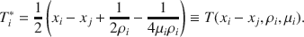
 . The results for optimal transfers are summarized in Table 2. Optimal transfers
 are unique except for the case where the subject i is not inequality averse (
 ) and cares about his own income as much as about his partner’s income (
 ).
).
Table 2 Optimal transfers as a function of
 and
and

|
Share of partner’s income |
Inequality aversion |
|
|---|---|---|
|
|
|
|
|
|
|
|
|
|
|
|
|
|
|
|
|
|
|
|


For
 and
and
 we have
 with
with

It is plausible to assume that subjects’ degree of inequality aversion is exogenous to the project’s payoffs and the experimental treatments, which is in line with our data.Footnote 16 For a given payoff difference and degree of inequality aversion, optimal transfers will depend on the weight of the partner’s income in the donor’s utility function,
 . Therefore, we model differences in other-regarding preferences across projects and treatments in terms of
 . Table 3 summarizes all possible constellations that we observe in the experiment. Let
 indicate subjects in RANDOM and
 subjects in CHOICE. Moreover, let
 denote donor’s project where
 for the safe project and
 for the risky project. Correspondingly, we denote partner’s project by
 . The combination of donor’s and partner’s project determines payoff levels and payoff differences.
For each treatment
 there are three combinations of donor’s project
 and partner’s project
 where the partner is worse off that correspond to three different combinations of donor’s and partner’s payoffs
 and
and
 . Moreover, a unique feature of the RANDOM treatment is that, due to randomization of projects, some subjects will unavoidably end up in a project that they would not choose for themselves. Let
 denote donor’s preferred project. In CHOICE, all subjects chose their preferred project such that actual and preferred project always coincide (
 ). Yet in RANDOM, there will always be a positive share of subjects where actual and preferred project differ (
 ). As a result, there are nine distinct groups in Table 3 that may differ in their other-regarding preferences
 . Therefore, we model
 flexibly as a function of all of these features:
 .
.
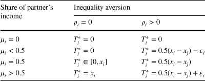
Table 3 Observed groups and optimal transfers when

|
Project of donor |
Project of partner |
Donor’s earnings |
Partner’s earnings |
Payoff difference |
||
|---|---|---|---|---|---|---|
|
Actual |
Preferred |
|||||
|
|
|
|
|
|
|
|
|
RANDOM not in preferred project (
|
||||||
|
(1) |
SAFE |
RISKY |
RISKY |
500 |
0 |
500 |
|
(2) |
RISKY |
SAFE |
SAFE |
1000 |
500 |
500 |
|
(3) |
RISKY |
SAFE |
RISKY |
1000 |
0 |
1000 |
|
RANDOM in preferred project (
|
||||||
|
(4) |
SAFE |
SAFE |
RISKY |
500 |
0 |
500 |
|
(5) |
RISKY |
RISKY |
SAFE |
1000 |
500 |
500 |
|
(6) |
RISKY |
RISKY |
RISKY |
1000 |
0 |
1000 |
|
CHOICE always in preferred project (
|
||||||
|
(7) |
SAFE |
SAFE |
RISKY |
500 |
0 |
500 |
|
(8) |
RISKY |
RISKY |
SAFE |
1000 |
500 |
500 |
|
(9) |
RISKY |
RISKY |
RISKY |
1000 |
0 |
1000 |


For given inequality aversion
 , it follows from equation (2) that optimal transfers increase with the payoff difference,
 , and the partner’s share in the utility function,
 . Thus, differences in transfers that we measure in the experiment are informative about differences in
 . Carpenter et al. (Reference Carpenter, Verhoogen and Burks2005) and Korenok et al. (Reference Korenok, Millner and Razzolini2012) show that transfers increase with the donor’s endowment, suggesting that
 . Moreover, Korenok et al. (Reference Korenok, Millner and Razzolini2012) show that the willingness to share income depends negatively on beneficiary’s income, for example because donors perceive individuals with higher income as less needy, suggesting that
 .
.
With our experiment we aim to test whether CHOICE of risk exposure affects the willingness to give compared to RANDOM assignment of risk exposure, i.e. whether
 . In particular, we hypothesize that this difference is negative. The notation already suggests that testing this hypothesis requires comparing subjects with the same preferred project. This is because the willingness to share income may also depend on risk preferences. For example, Cettolin and Riedl (Reference Cettolin and Riedl2017) and Cettolin et al. (Reference Cettolin and Tausch2017) show that risk preferences correlate with other-regarding preferences. Moreover, the subjects in RANDOM who end up in a project that they would not choose for themselves (
 ) face a utility loss compared to assignment to their preferred project. Hence, they may find it optimal to lower transfers to compensate for this utility loss.
If transfers indeed depend on preferred projects, then comparing average transfers across treatments no longer provides a valid test of the hypothesis that CHOICE reduces transfers compared to RANDOM. This is because for subjects in RANDOM who are not in their preferred project there are no comparable subjects in CHOICE as all subjects are in their preferred project in CHOICE. We can exploit, though, that whether or not a subject in RANDOM ends up in his or her preferred project is random. As a result, we can compare transfers across treatments conditional on being in one’s preferred project to obtain a valid test of the hypothesis that CHOICE reduces transfers compared to RANDOM. This, however, requires eliciting subjects preferred project in RANDOM, which we do in our experiment.
Another advantage of conditioning on being in one’s preferred project is that it enables us to compare the effect of CHOICE for different combinations of donor’s and partner’s project. This, in turn, allows us to discriminate between different possible explanations for reduced transfers, as we discuss in the next section. Without the ability to align project preferences across treatments, comparing transfers of subjects with the same project across treatments is flawed by selection bias that results from the fact that subjects who chose a given project in CHOICE systematically differ from the subjects randomly assigned to the same project in RANDOM.
3.2 Hypotheses
In the following, we derive five hypotheses that are directly testable with our experimental design. We summarize them and the comparisons they require in Table 4. The first hypothesis refers to our methodological point that the presence of subjects in projects they would not choose in RANDOM invalidates average transfers in RANDOM as a valid counterfactual. A sufficient condition for the difference in average transfers across treatments leading to a biased estimate of the effect of CHOICE of interest is that average transfers in RANDOM differ for subjects randomly assigned to their preferred project and subjects randomly assigned to an unwanted project:
Hypotheses H1
(Assignment to unwanted projects in RANDOM matters for transfers) Subjects who are assigned to their preferred project in RANDOM on average make different transfers than subjects who are assigned to an unwanted project in RANDOM.
With the second hypothesis we aim to test whether previous findings of reduced solidarity for Western countries and of crowding out of informal support by the availability of formal insurance in developing countries extend to more general situations that include opting into risk in developing countries. Therefore, we hypothesize that:
Hypotheses H2
(CHOICE reduces transfers) Average transfers in CHOICE are lower than average transfers of subjects assigned to their preferred project in RANDOM.
If the data confirm hypothesis 2, we still do not know the behavioural mechanism behind lower transfers in CHOICE. Therefore, we want to test for three possible channels through which CHOICE may reduce transfers. The first one is attributions of responsibility for neediness in CHOICE that is motivated by a shared norm about low risk-taking, which is the main channel advocated by previous research. Since subjects can avoid income risk by choosing the safe project, we expect that CHOICE reduces transfers to partners who choose the risky project but not to partners who choose the safe project if attributions of responsibility for neediness are the main motive. Transfers to partners choosing the safe project should either be unaffected by CHOICE in this case; or safety choosers may even be rewarded for abiding by the shared norm of low risk-taking with higher transfers in CHOICE than in RANDOM. Thus, we expect a non-negative effect of CHOICE on transfers to safety choosers. We summarize these predictions in the following hypothesis:
Hypotheses H3
(Attributions of responsibility) If attributions of responsibility for neediness drive donors’ transfer choices, then transfers to partners with the risky but not with the safe project are lower in CHOICE than in RANDOM.
An alternative explanation for reduced transfers in CHOICE is a higher willingness to share income received by pure luck than income received as the result of a deliberate choice. For example, donors who receive a payoff of 1000 KSh with the risky project by pure chance in RANDOM may feel a stronger obligation to share this high payoff than donors who realize the same payoff because of a deliberate decision to take risk in CHOICE. This is because everybody had the chance to pick the risky project and be lucky in CHOICE but not in RANDOM. Borrowing from the terminology used by Cappelen et al. (Reference Cappelen, Konow, Sorensen and Tungodden2013), one could call this a form of ex-ante choice egalitarianism. It is a form of ex-ante fairness perception that is only present if subjects can choose risk exposure. Because everybody had the possibility to make the same choice ex ante, donors may feel entitled to keeping their money independent of the partner’s choice and realized outcome. The same behaviour can be motivated by the view that partners who choose the safe project in CHOICE signal that they are happy with 500 KSh, while partners who choose the risky project accept the possibility of receiving nothing. Hence, donors may feel that partners expect less because they are fine with their choice. Thus, if ex-ante choice egalitarianism drives behaviour, then we expect donors to reduce transfers independent of their own and their partner’s choice:
Hypotheses H4
(Ex-ante choice egalitarianism) Under ex-ante choice egalitarianism, donors make lower transfers in CHOICE than in RANDOM independent of their own and their partner’s choice.
The last explanation for reduced transfers in CHOICE we can test with our experimental design is ex-post choice egalitarianism as discussed by Cappelen et al. (Reference Cappelen, Konow, Sorensen and Tungodden2013). Under ex-post choice egalitarianism, subjects view income inequalities as fair if they result from different choices but as unfair if they are due to different outcome realizations that result from the same choice. As subjects cannot choose their project in RANDOM, such a distinction should be absent in RANDOM. Hence, transfers should be lower in CHOICE than in RANDOM when donor’s and partner’s choice differ but not when they are the same:
Hypotheses H5
(Ex-post choice egalitarianism) Transfers in CHOICE are lower than in RANDOM when donor’s and partner’s choice differ but not when they are the same.
Table 4 Hypotheses
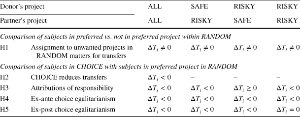
|
Donor’s project |
ALL |
SAFE |
RISKY |
RISKY |
|
|---|---|---|---|---|---|
|
Partner’s project |
ALL |
RISKY |
SAFE |
RISKY |
|
|
Comparison of subjects in preferred vs. not in preferred project within RANDOM |
|||||
|
H1 |
Assignment to unwanted projects in RANDOM matters for transfers |
|
|
|
|
|
Comparison of subjects in CHOICE with subjects in preferred project in RANDOM |
|||||
|
H2 |
CHOICE reduces transfers |
|
– |
– |
– |
|
H3 |
Attributions of responsibility |
|
|
|
|
|
H4 |
Ex-ante choice egalitarianism |
|
|
|
|
|
H5 |
Ex-post choice egalitarianism |
|
|
|
|


We can test all hypotheses in Table 4 directly with the experimental data by comparing average transfers in the respective groups under the assumption that we correctly measure preferred projects
 in RANDOM. We discuss the validity of this assumption and other aspects of our experimental design in the following.
4 Does our experimental design work?
4.1 Did randomization work?
To obtain unbiased estimates we need to make sure that randomization into treatments and into projects within RANDOM created comparable groups. In Table 10 in online Appendix A, we report the means of all variables in our data by treatment and by project within treatment. Randomization of treatments worked very well. The majority of means is very similar. For only 2 out of 50 variables we find differences that are significant on the 10% level. The randomization of projects within RANDOM also succeeded in creating comparable groups with only 3 out of 50 differences in means being significant on the 10% level. For CHOICE, Table 10 in online Appendix A shows the selectivity of project choice. Subjects who choose the risky project have a much stronger preference for risk as expected, higher income, fewer other earners in the household, and they are more likely to be the household head, where the latter is explained by a higher share of males.
4.2 Do we correctly measure preferred projects in RANDOM?
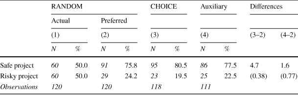
Given that randomization worked very well, the most crucial part of our experiment is whether we correctly measure preferred projects for subjects in RANDOM. One major concern could be that subjects in RANDOM only answer a hypothetical question without any monetary consequences, whereas the subjects in CHOICE have to face the consequences of their choice. Another concern is that we elicit preferences ex post after transfer decisions have been made. There are several ways to assess whether there are any systematic differences in the preferences stated by the subjects in RANDOM compared to those in CHOICE. As a first check, we compare the share of subjects preferring the risky project in CHOICE and RANDOM. In CHOICE, 19.5% of subjects choose the risky project whereas in RANDOM 24.2% prefer it. The difference is not statistically significant with a p-value of .38 (see Table 5).
Table 5 Distribution of projects by treatment
|
RANDOM |
CHOICE |
Auxiliary |
Differences |
|||||||
|---|---|---|---|---|---|---|---|---|---|---|
|
Actual |
Preferred |
|||||||||
|
(1) |
(2) |
(3) |
(4) |
(3–2) |
(4–2) |
|||||
|
N |
% |
N |
% |
N |
% |
N |
% |
|||
|
Safe project |
60 |
50.0 |
91 |
75.8 |
95 |
80.5 |
86 |
77.5 |
4.7 |
1.6 |
|
Risky project |
60 |
50.0 |
29 |
24.2 |
23 |
19.5 |
25 |
22.5 |
(0.38) |
(0.77) |
|
Observations |
120 |
120 |
118 |
111 |
||||||
P-values in parentheses
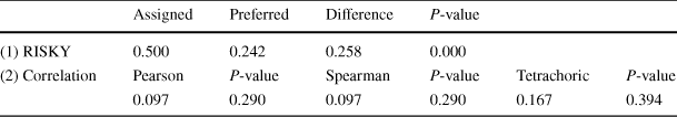
As a second check, we test whether subjects rationalize the project they have been assigned to in RANDOM when stating their preferred project ex post. To do so, we firstly, check for a statistically significant difference in the share being assigned to and preferring the risky project in RANDOM in line (1) of Table 6. The difference is 25.8 percentage points and highly statistically significant. Secondly, we test for a positive correlation between assigned and preferred project in RANDOM in line (2) of Table 6. The correlations are positive but small and not statistically significant with p-values around 30%. Hence, we cannot reject the hypothesis that assigned and preferred projects are uncorrelated in RANDOM.
Table 6 Relation between assigned and preferred projects in RANDOM
|
Assigned |
Preferred |
Difference |
P-value |
|||
|---|---|---|---|---|---|---|
|
(1) RISKY |
0.500 |
0.242 |
0.258 |
0.000 |
||
|
(2) Correlation |
Pearson |
P-value |
Spearman |
P-value |
Tetrachoric |
P-value |
|
0.097 |
0.290 |
0.097 |
0.290 |
0.167 |
0.394 |
The third check compares the characteristics of the subjects preferring the same project across the two treatments. These should not differ systematically because subjects with the same characteristics should on average state the same preference in CHOICE as in RANDOM if preferences are measured correctly. In Table 10 in online Appendix A we report the means of all variables by chosen project in CHOICE and by preferred project in RANDOM, and we test for statistically significant differences between the two. For subjects who prefer the safe project, only 3 out of 50 differences in means are significant on the 10% level and 2 of them correspond to the ones for which we find small sample imbalances between RANDOM and CHOICE in general. For subjects who prefer the risky project, there are only 2 statistically significant differences in means on the 5% level which is to be expected with 50 variables tested. In Table 11 in online Appendix A we additionally report the same statistics conditional on assigned project in RANDOM. Specifically, we compare subjects with the safe project in CHOICE with the subgroup of subjects assigned to the safe project in RANDOM that also prefers the safe project and correspondingly for the risky project. These are the groups that will be used for the estimation. For both the safe and the risky project we only find one variable with a difference in means that is significant on the 10% level. Thus, we can conclude that subjects in CHOICE and RANDOM who state to prefer the same project do not differ systematically in the large number of observed drivers of project choice and willingness to give.
The fourth check makes use of the auxiliary experiment, where all subjects choose between the safe and the risky project as in CHOICE but without running the solidarity game. This addresses two possible concerns. Firstly, we can assess whether real monetary consequences matter for stated preferences. In the auxiliary experiment but not in RANDOM, project choice is incentivized as it determines subjects’ payoff from the experiment. Secondly, we can address the issue that subjects may choose projects strategically in CHOICE because they know that they have to make a decision on transfers to worse-off partners after having chosen a project. This is because the probability to face a partner who is worse off differs by project.Footnote 17 This would imply that project choice is determined by other factors than risk preferences in CHOICE. If we find no systematic differences between the distributions of stated preferences and the characteristics of subjects with the same stated preference between the auxiliary experiment and each of the two treatment groups in the main experiment, then this is supporting evidence for the validity of our experimental design.
In Table 12 in online Appendix A, we report the means of all variables for the subjects in RANDOM and in the auxiliary experiment, as well as in the subgroups that state to prefer the safe and the risky project, respectively. The subjects we sampled for the auxiliary experiment are somewhat better educated than the ones we sampled for the main experiment, which results in lower rates of unemployment and higher wealth, and which is correlated with ethnicity. Other than that, there are 3 more statistically significant means which do not show a systematic pattern, though. Apart from these small sample imbalances we do not find any systematic differences between subjects with the same stated preferences, though. The share of subjects preferring the risky project in the auxiliary experiment is 22%, which is 1.6 percentage points lower than in RANDOM with the difference being not statistically different from zero at a p-value of .77 (see Table 5). Differences in mean characteristics of safety choosers between the main and the auxiliary experiment only mirror the sample imbalances. The findings for risk takers are similar with only few statistically significant differences in means that mostly mirror the sample imbalances. There are only 2 out of 50 variables with significant difference that are not directly related to the sample imbalances. Thus, the auxiliary experiment does not provide any evidence for systematic differences in stated preferences to subjects in RANDOM, and for them, we do not find systematic differences compared to CHOICE. This, together with the other evidence presented above, makes us very confident that we correctly measure preferred projects for all subjects and that project choices reflect risk preferences.
5 Results
5.1 Giving behaviour and implied preferences
Before turning to the hypotheses, we discuss what observed transfers in the experiment tell us about the underlying sharing norms and other-regarding preferences. In Table 13 in online Appendix B we report mean transfers for all observed groups of subjects in the data. We find that, on average, donors give away 202 KSh in RANDOM and 157 KSh in CHOICE. With their gifts, they offset 31.3% and 28.2% of the payoff differences, respectively. The partner’s average final share of the pair’s aggregated income,
 , is 34% in RANDOM and 32% in CHOICE. This finding is well in line with the majority of results of dictator game experiments conducted in rural Kenya, whose sharing task might be comparable to that in our RANDOM treatment. For example, Ensminger (Reference Ensminger and Ménard2000) finds a mean offer of 31% and Henrich et al. (Reference Henrich, McElreath, Barr, Ensminger, Barrett, Bolyanatz, Cardenas, Gurven, Gwako, Henrich, Lesorogol, Marlowe, Tracer and Ziker2006) of 33% to 40%.Footnote 18 Moreover, this is considerably larger than comparable results for Western countries. For example, Cappelen et al. (Reference Cappelen, Konow, Sorensen and Tungodden2013) report 24% for Norway. Cardenas and Carpenter (Reference Cardenas and Carpenter2008) summarize the results from dictator games conducted in different countries. For developing countries, most results are well above 30% as in our experiment. In contrast, for Western countries such as the United States, Russia and Sweden most results are well below 30%. This supports our claim of a stronger social norm towards sharing in developing countries.
Nevertheless, a substantial part of the subjects decided to give nothing to their partner. On average, the cases of zero transfers account for nearly 40% in both treatments. These subjects either place no weight on their partner’s income in their utility function such that
 , or they are not inequality averse such that
 , and have
 . A share of 31% (36%) of subjects in RANDOM (CHOICE) make positive transfers but give less than half of the payoff difference to their partner. This is in line with subjects being inequality averse (
 ) and giving less than equal weight to the partner’s payoff in the utility function (
 ). A share of 17.2% (12.1%) of the subjects in RANDOM (CHOICE) follow an equal sharing rule, which implies that they are inequality averse,
 , and that they place equal weights on their own and their partner’s income in their utility function,
 .Footnote 19 Few subjects place more weight on their partner’s than on their own income,
 , and give away more than half of the payoff difference. In total, 25–30% of subjects do not give less to the partner than they keep for themselves. This is in line with the share agreeing to the statement that others should not own much less than they do (see Table 1).
5.2 Does project preference matter for transfers in RANDOM?
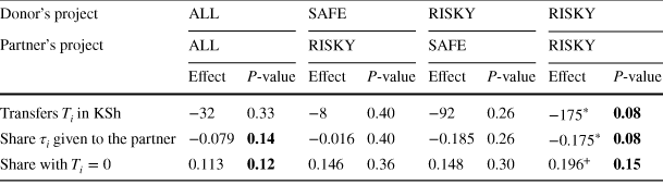
We argue that the fact that some subjects in RANDOM end up in projects they would not choose for themselves invalidates average transfers in RANDOM as suitable comparison to average transfers in CHOICE, where all subjects are in their preferred project by construction. This is the case if subjects who are assigned to their preferred project in RANDOM make different transfers than subjects who are assigned to an unwanted project in RANDOM, which is what we state in hypothesis H1. Figure 2 shows average giving behaviour in RANDOM by whether or not subjects are in their preferred project. In line with H1, we find that donors in their preferred project give more to their partners than donors in an unwanted project.
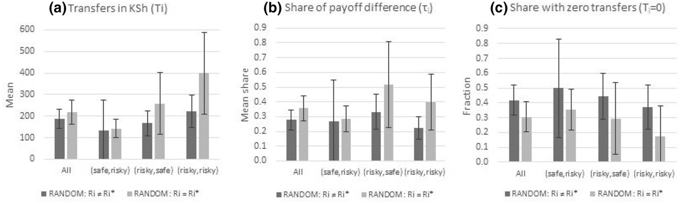
Fig. 2 Average giving behaviour in RANDOM by project preference. Note: The figure contrasts transfers in RANDOM for subjects in non-preferred versus preferred projects with 95% confidence bands. Donor’s (left) and partner’s project (right) are indicated in parentheses. Transfers are measured in Kenyan shillings (left panel), as share of payoff difference between donor and partner (middle panel), and as share of subjects making zero transfers (right panel).
 measures the share of the payoff difference given to the partner
Table 7 presents formal tests for zero differences in giving. Inference is based on the wild bootstrap (Wu Reference Wu1986) with 999 replications and null imposed, as recommended by Cameron et al. (Reference Cameron, Gelbach and Miller2008) for estimates with clustered standard errors and few clusters. This accounts for the fact that randomization into treatments takes place on the session level. Additionally, we present p-values from non-parametric Wilcoxon rank-sum tests for differences in the distributions of transfers. This provides a more general test of the hypothesis that transfers differ across groups.Footnote 20 We find that the differences we observe in Fig. 2 are statistically significant in many cases, which supports hypothesis H1. Moreover, the results suggest that donors may indeed reduce transfers to compensate utility losses associated with assignment to an unwanted project. They imply further, that conditioning on preferred projects is crucial for isolating the effects of CHOICE and that naïvely comparing mean transfers across treatments would underestimate negative effects of CHOICE.
Table 7 Effect of being assigned to an unwanted project in RANDOM
|
Donor’s project |
ALL |
SAFE |
RISKY |
RISKY |
||||
|---|---|---|---|---|---|---|---|---|
|
Partner’s project |
ALL |
RISKY |
SAFE |
RISKY |
||||
|
Effect |
P-value |
Effect |
P-value |
Effect |
P-value |
Effect |
P-value |
|
|
Transfers
|
−32 |
0.33 |
−8 |
0.40 |
−92 |
0.26 |
−175
|
0.08 |
|
Share
|
−0.079 |
0.14 |
−0.016 |
0.40 |
−0.185 |
0.26 |
−0.175
|
0.08 |
|
Share with
|
0.113 |
0.12 |
0.146 |
0.36 |
0.148 |
0.30 |
0.196
|
0.15 |


The table shows the difference in average giving between subjects in an unwanted project in RANDOM (
 ) and subjects in their preferred project (
 ).
).
 measures the share of the payoff difference given to the partner.
 indicates significance on the 1/5/10/15% level based on 999 Wild bootstrap replications. P-values stem from non-parametric Wilcoxon rank-sum tests and are marked with bold font if
 15%
15%
5.3 Does deliberate choice of risk reduce transfers?
In Figure 3 we compare average giving behaviour of subjects in their preferred project across the CHOICE and RANDOM treatments as test of the hypothesis that choice of risk reduces willingness to give. We see only moderate negative effects of CHOICE on transfers when we pool all subjects. However, we find relatively large reductions of transfers by donors in the risky project, which make up about 20% of our sample. We also find that these reductions do not differ by partner’s project.
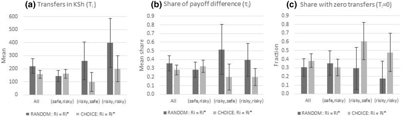
Fig. 3 Average giving behaviour of subjects in their preferred project by treatment. Note: The figure compares transfers in RANDOM vs. CHOICE using only subjects in their preferred projects with 95% confidence bands. Donor’s (left) and partner’s project (right) are indicated in parentheses. Transfers are measured in Kenyan shillings (left panel), as share of payoff difference between donor and partner (middle panel), and as share of subjects making zero transfers (right panel).
 measures the share of the payoff difference given to the partner
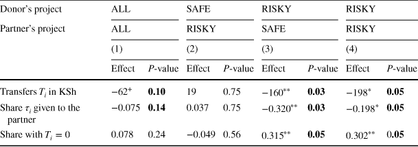
In Table 8 we formally test for effects of CHOICE.Footnote 21 The overall negative effects of CHOICE on transfers in column (1) are relatively small with -62 KSh and only marginally statistically significant. Thus, we find only weak support for hypothesis H2 that CHOICE reduces average transfers. The small average effect results from donors preferring the safe project who are paired with partners in the risky project. They account for about 80% of subjects and for them CHOICE has no statistically significant effect on transfers in column (2). Hence, they neither punish partners for exposing themselves to risk, rejecting attributions of responsibility (H3), nor do they give less independent of the partner’s choice due to same ex-ante choice opportunities, rejecting ex-ante choice egalitarianism (H4), nor do they punish partners for choosing a project that differs from their own choice, rejecting ex-post choice egalitarianism (H5) as well. Thus, our results support none of the hypotheses about the effects of CHOICE for safety choosers.
Table 8 Effects of CHOICE on giving for subjects in their preferred project
|
Donor’s project |
ALL |
SAFE |
RISKY |
RISKY |
||||
|---|---|---|---|---|---|---|---|---|
|
Partner’s project |
ALL |
RISKY |
SAFE |
RISKY |
||||
|
(1) |
(2) |
(3) |
(4) |
|||||
|
Effect |
P-value |
Effect |
P-value |
Effect |
P-value |
Effect |
P-value |
|
|
Transfers
|
−62
|
0.10 |
19 |
0.75 |
−160
|
0.03 |
−198
|
0.05 |
|
Share
|
−0.075 |
0.14 |
0.037 |
0.75 |
−0.320
|
0.03 |
−0.198
|
0.05 |
|
Share with
|
0.078 |
0.24 |
−0.049 |
0.56 |
0.315
|
0.05 |
0.302
|
0.05 |


The table shows the difference in average giving of subjects in their preferred project between CHOICE and RANDOM.
 measures the share of the payoff difference given to the partner.
 indicates significance on the 1/5/10/15% level based on 999 Wild bootstrap replications. P-values stem from non-parametric Wilcoxon rank-sum tests and are marked with bold font if
 15%
15%
In contrast, donors choosing the risky project give considerably less to their partners in CHOICE than in RANDOM. On average, they reduce transfers by 160-200 KSh. The share of the payoff difference given to the partner falls by 20-30 percentage points and the share with zero transfers increases by 30 percentage points. The magnitude of the negative effects of CHOICE is only slightly larger for partners who self-select into the risky project in column (4) than for partners choosing the safe project in column (3), and we do not reject equality of the effects (see line (13) of Table 14) in online Appendix B. As a result and in line with the findings for donors choosing the safe project, we reject both attributions of responsibility for neediness (H3), and ex-post choice egalitarianism (H5) as the main explanations for reduced transfers in CHOICE. Instead, our findings support ex-ante choice egalitarianism (H4) in the group of risk-takers. It predicts that donors in the risky project feel a stronger obligation to share the high payoff of 1000 KSh when they received it by pure luck in RANDOM than in a situation that involves a deliberate decision for the risky project. This is because ex-ante, everybody had the chance to pick the risky project and be lucky in CHOICE but not in RANDOM.
The result that attributions of responsibility for neediness do not explain reduced transfers in CHOICE is an interesting finding, because it deviates from the previous findings of reduced solidarity for Western countries and of crowding out of informal support by the availability of formal insurance in developing countries. The latter suggests that fairness views regarding risk avoidance may differ from those regarding opting into risk with the potential of realizing higher payoffs that may benefit risk-sharing partners. Compared to Western countries, our results suggests that the importance of informal insurance for the poor population, the strong sharing norms rooted in African cultures and the overall high risk exposure in developing countries might reduce the sensitivity of subjects’ solidarity with respect to others’ risk-taking.
Our finding that donors’ behaviour depends on risk preferences is in line with Cettolin and Riedl (Reference Cettolin and Riedl2017) and Cettolin et al. (Reference Cettolin and Tausch2017). In Table 9, we further explore possible explanations for this finding. Here, we report mean transfers that donors expected to receive from their partners had they been worse off. We find that donors’ behaviour mirrors their own expectations regarding transfers from others. Safety choosers in CHOICE expect the same transfers from their counterparts as in RANDOM. Risk-takers, however, expect significantly less from their partners, especially when the partner also takes risk.Footnote 22 This suggests, that risk choosers take responsibility for their decision by expecting less from others, especially from other risk takers. In return, though, they are less willing to share high payoffs with worse-off partners.
Table 9 Difference in average transfers expected from better-off partners
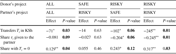
|
Donor’s project |
ALL |
SAFE |
RISKY |
RISKY |
||||
|---|---|---|---|---|---|---|---|---|
|
Partner’s project |
ALL |
RISKY |
SAFE |
RISKY |
||||
|
Effect |
P-value |
Effect |
P-value |
Effect |
P-value |
Effect |
P-value |
|
|
Transfers
|
−71
|
0.03 |
−14 |
0.63 |
−102
|
0.06 |
−245
|
0.01 |
|
Share
|
−0.081 |
0.09 |
−0.027 |
0.63 |
−0.204
|
0.06 |
−0.245
|
0.01 |
|
Share with
|
0.129
|
0.04 |
0.055 |
0.46 |
0.243
|
0.12 |
0.317
|
0.03 |


The table shows the difference in average expected giving from better-off partners in their preferred project between CHOICE and RANDOM.
 measures the share of the payoff difference given to the partner.
 indicates significance on the 1/5/10/15% level based on 999 Wild bootstrap replications. P-values stem from non-parametric Wilcoxon rank-sum tests and are marked with bold font if
 15%
15%
These findings are in line with D’Exelle and Verschoor (Reference De Mel, McKenzie and Woodruff2015) who study investment behavior and risk sharing in a lab-in-the-field experiment in Uganda. They find that individuals who make risky investments share less of both their profits, and their losses. They argue that investors may consider it to be unfair if other people share a substantial part of the loss of their risky investment if it failed. At the same time, investors may consider it to be unfair if they have to share a substantial part of the profits if the investment was successful. This implies that investors are aware of the burden their investment behavior may impose on others in societies with a strong social norm towards sharing while at the same time feeling less obliged to share the profits they make out of these investments. Our results show in addition that individuals who prefer to avoid risky situations expect and provide a certain level of support independent of the situation that has put them on either the giving or receiving end in such societies.
6 Conclusion
This study investigates whether solidarity, which is a crucial base for informal insurance arrangements in developing countries, is sensitive to the extent to which individuals can influence their risk exposure. In a laboratory experiment with slum dwellers in Nairobi we measure subjects’ transfers to a worse-off partner in a setting where participants could either deliberately choose (treatment CHOICE) or were randomly assigned (treatment RANDOM) to a safe or a risky project. In contrast to previously conducted experiments that study similar questions, we use an experimental design that elicits preferred projects for all subjects. This allows us to separate the effect of CHOICE on fairness views from other differences across treatments and to discriminate between three different possible explanations for why giving behaviour might change when risk exposure is self-selected rather than exogenous.
We find that free choice of risk exposure reduces transfers. However, in line with Cettolin and Riedl (Reference Cettolin and Riedl2017) and Cettolin et al. (Reference Cettolin and Tausch2017) we find that the response depends on risk preferences. We find that the reduction in transfers is limited to donors who prefer the risky project and it is independent of the partner’s choice of project. As a result, we reject attributions of responsibility for neediness as explanation for reduced transfers. As donors also do not make their transfers dependent on whether income inequalities result from different choices or different outcome realizations of the same choice, we also reject ex-post choice egalitarianism. Instead, we find that donors in the risky project feel a stronger obligation to share the high payoff when they received it by pure luck in RANDOM than in the situation when receiving it involves a deliberate decision for the risky project. This is in line with a form of ex-ante choice egalitarianism that views income inequalities as fair if everybody had the same chance to pick a specific project as in CHOICE but not if this option does not exist as in RANDOM. In line with D’Exelle and Verschoor (Reference De Mel, McKenzie and Woodruff2015), we also find that risk choosers seem to take responsibility for their own risky choice by expecting less from others in case they end up with nothing.
Overall it seems that the strong norm of mutual support in developing countries works against strong punishment of risky choices and makes risk choosers aware of the burden their investment behavior may impose on others. In this respect, our findings differ substantially both from the evidence for Western countries (Trhal and Radermacher Reference Trhal and Radermacher2009; Cettolin and Tausch Reference Cettolin, Riedl and Tran2015; Akbas et al. Reference Akbas, Ariely and Yuksel2019), and the evidence on crowding out of informal insurance by the availability of formal insurance for developing countries (Landmann et al. Reference Landmann, Vollan and Froelich2012; Lin et al. Reference Lin, Liu and Meng2014; Anderberg and Morsink Reference Amendah, Buigut and Mohamed2020; Lenel and Steiner Reference Lenel and Steiner2020). Since we study the situation where subjects can opt into risky income opportunities instead of opting out of risk via insurance, our results suggest that not only the social norm regarding solidarity in a society matters, but also the situation in which individuals make choices that involve risk. Future research should investigate how sharing behaviour in developing countries depends on the stakes involved in different investment opportunities, repeated and strategic interactions between donors and recipients, as well as how subjects under random risk allocation interact with subjects under choice of risk.
Our findings have important implications for policies that aim to encourage entrepreneurship or investments into new but risky business opportunities to reduce poverty and foster economic growth in developing countries. They suggest that crowding out of informal support by subjects who prefer not to engage in these activities may actually not be an issue. Moreover, negative effects on overall solidarity in a society will depend on the share of individuals who make use of these risky opportunities. The larger this share is, the more likely it is that crowding out of informal support by other risk takers has notable effects on overall support for these activities, which would counteract the intention of these policies. This suggests that there should exist an optimal level of encouragement of risk-taking at which the cost in terms of reduced support by others is not too high.
Acknowledgements
We thank the team of the Busara Center of Behavioral Economics in Nairobi, in particular Chaning Jang, Georgina Mburu, Lucy Rimmington, Arun Varghese and all involved research assistants for helping to realize this project and their support. Moreover, we thank seminar participants at the Universities of Basel, Göttingen, Hannover, Lucerne, Lugano, Neuchatel, Mannheim and Munich as well as participants at various conferences for helpful discussions and comments. Working papers summarizing earlier output from this project circulated under the titles “Does Voluntary Risk Taking Affect Solidarity? Experimental Evidence from Kenya” and “Risky Choices and Solidarity: Why Experimental Design Matters”. The current paper replaces both papers.
Funding
Open Access funding provided by University of Basel.
Compliance with ethical standards
Conflict of interest
The author declares that there is no conflict of interest.


 μi
μi ρi
ρi
 μi,ρi>0


 τi=Ti/(xi-xj)

 τi=Ti/(xi-xj)


 Open access