


Many economic decisions involve a trade-off between benefits and costs in the present and in the future: how much to consume versus save for later, whether to exercise or not, and whether to complete an onerous task today or to postpone it. These decisions involve individuals making choices at multiple points in time with no ability to commit to future choices. Until recently, most intertemporal choice experiments only studied choices over delayed monetary rewards made at a single point in time (e.g. Coller & Williams Reference Coller and Williams1999; Harrison et al. Reference Harrison, Lau and Williams2002; Andreoni & Sprenger Reference Andreoni and Sprenger2012). As a result, economists have limited experimental evidence on time inconsistency for non-monetary rewards and even less evidence on how people form expectations about their own future time inconsistency. We contribute by studying participants’ decisions to complete a task or delay in an environment without commitment in order to reveal their sophistication about their own time inconsistency.
We introduce a multi-day experimental design to observe task completion decisions over real effort and time. Each participant must complete a real effort task that consists of a number of chores to be eligible for a fixed payment at the end of the week. Crucially, a participant’s initial choices cannot commit their future choices except by completing the task. Each participant is presented with multiple two-date and three-date effort schedules that specify the number of chores associated with each of the available dates. For each effort schedule that includes the current day, the participant must indicate their choice to either do the task “today” or “not today”. If they choose “today”, they must complete the specified number of real effort chores by the end of today to be eligible for payment. If they choose “not today”, then the next day they face all effort schedules for which they previously selected “not today” plus those schedules for which “today” was not previously available. Across schedules we vary both the effort required on each available day and the days available to complete the task. In each two-date schedule, each decision at the earlier date elicits a preference at the earlier date. In each three-date schedule, each decision at the earlier date reflects both preferences and expectations about future behavior. Combining observations from two- and three-date effort schedules allows us to test axioms about intertemporal preferences and expectations about future preferences using choice data.
Our experiment is designed to test three normative axioms of intertemporal choice: sophistication, time consistency and time invariance. The sophistication axiom requires that a person correctly forecasts their future choices. The time consistency axiom requires that if a person chooses an option over another today, they would wish to make that same choice between options tomorrow if the consequences of the two actions have not changed. The time invariance axiom requires that if a person chooses one option over another today, they would make the same choice tomorrow if the consequences of each action were shifted one day in the future (Halevy, Reference Halevy2015). Each of the three axioms restricts the relationship between choices at two points in time, and there is limited body of experimental work that tests them using choices. Our design uses combinations of two- and three-date effort schedules that allow us to test each axiom for each experiment participant.
We find that participants demonstrate a tendency to complete a task immediately, even when delaying would have reduced the number of required chores. Specifically, 78% of two-date choices are resolved in favor of completing the task immediately, including 52% of two-date choices in which delaying reduces the number of chores. In two-date choices a participant’s beliefs about their future behavior are trivial and thus the immediate completion tendency we document for real effort tasks does not arise from sophistication about inconsistent preferences. Participants exhibit a high degree of time consistency despite the considerable power of our experiment to detect violations of this axiom. We find that 50 of 82 participants are time consistent in every test, and 29 of these 50 always choose to complete the task on Day 1 when it is available regardless of the effort trade-off.
We discuss how our findings relate to several theories of intertemporal choice. A structural model of quasi-hyperbolic discounting requires a future bias (
 ) to capture the early completion tendency we observed, which contradicts the intuition that people prefer to delay unpleasant tasks (e.g. O’Donoghue & Rabin Reference O’Donoghue and Rabin1999). Our design controls for fixed costs with a daily login requirement, equalizes costs of keeping track by using reminders, and we show that decision costs cannot rationalize our findings. A model of anticipatory utility like that of Loewenstein (Reference Loewenstein1987) can generate an early completion tendency, but we show that the assumptions required would incorrectly predict an early completion tendency in the convex time budget (CTB) experiments of Augenblick et al. (Reference Augenblick, Niederle and Sprenger2015). A model in which a person discounts future goods and bads by a subjective and fixed amount, i.e., a subjective fixed cost of delay (Hardisty et al., Reference Hardisty, Appelt and Weber2013) can generate present bias for goods and an immediate completion tendency for bads like real effort tasks (though our design controls for actual fixed costs). An alternative explanation is that people are biased to get tasks started, as seen in some psychology experiments following Rosenbaum et al. (Reference Rosenbaum, Gong and Potts2014). Our results suggest that intertemporal choices are affected by a factor distinct from present bias that is amenable to behavioral modeling.
Related Literature There is an extentsive experimental literature on intertemporal choice that studies preferences over delayed monetary rewards revealed at one point in time (e.g. Coller & Williams Reference Coller and Williams1999; Harrison et al. Reference Harrison, Lau and Williams2002). Since money can be saved and borrowed such experiments should not, in principle, reveal intertemporal preferences if participants broadly bracket their experimental choices with opportunities outside of the lab (Cubitt & Read, Reference Cubitt and Read2007; Cohen et al., Reference Cohen, Ericson, Laibson and White2020). Thus, some intertemporal choice experiments use less-fungible rewards that will be consumed immediately like snacks (Read et al., Reference Read and Van Leeuwen1998)) and real effort tasks (Augenblick et al., Reference Augenblick, Niederle and Sprenger2015; Carvalho et al., Reference Carvalho, Meier and Wang2016; Augenblick, Reference Augenblick2018; Augenblick & Rabin, Reference Augenblick and Rabin2019; Le Yaouanq & Schwardmann, Reference Le Yaouanq and Schwardmann2019; Bisin & Hyndman, Reference Bisin and Hyndman2020; Breig et al., Reference Breig, Gibson and Shrader2020; Hardisty & Weber, Reference Hardisty and Weber2020; Fedyk, Reference Fedyk2021; Zou, Reference Zou2021)). Most papers in this literature find that subjects are present biased on average, a finding less pronounced for monetary rewards (Augenblick et al., Reference Augenblick, Niederle and Sprenger2015); see also meta studies by Imai et al. (Reference Imai, Rutter and Camerer2020) and Cheung et al. (Reference Cheung, Tymula and Wang2021)). Our design uses a real effort task from Augenblick et al. (Reference Augenblick, Niederle and Sprenger2015).
Several papers in this literature indirectly test for a person’s sophistication or naivete about their own time inconsistency by measuring demand for commitment devices (e.g. Ashraf et al. Reference Ashraf, Karlan and Yin2006; Augenblick et al. Reference Augenblick, Niederle and Sprenger2015; see a review in Bryan et al. (Reference Bryan, Karlan and Nelson2010)) or by comparing elicited beliefs to actual future choices (Augenblick & Rabin, Reference Augenblick and Rabin2019; Hardisty & Weber, Reference Hardisty and Weber2020)). In contrast, our design elicits choices at different points in time in an environment where a participant cannot commit their future choices. This allows us to employ Freeman’s (Reference Freeman2021) approach to test both sophistication and naivete about time inconsistency for each participant. Our design is motivated by a literature that commonly finds evidence of time inconsistency and that has found widely different degrees of sophistication about it (Ashraf et al., Reference Ashraf, Karlan and Yin2006; Augenblick et al., Reference Augenblick, Niederle and Sprenger2015; Augenblick & Rabin, Reference Augenblick and Rabin2019)). Yet, unlike this literature, we find little evidence of time inconsistency and thus have little to say about sophistication and naivete.
Most of the earlier literature on intertemporal choice only studies choices made at one point in time and thus cannot directly test time consistency or time invariance, with some exceptions,Footnote 1 For instance, Read et al. (Reference Read and Van Leeuwen1998) have their participants choose a post-lunch snack both a week in advance and again the day they consume the snacks. They find participants choose unhealthy snacks more frequently when choosing same-day than in-advance. Augenblick et al. (Reference Augenblick, Niederle and Sprenger2015) study participants’ allocations of real effort chores between earlier and later dates, both when the earlier date is in the future and when it is immediate. Similarly, Augenblick and Rabin (Reference Augenblick and Rabin2019) elicit participant preferences over quantities of delayed real effort chores at different points in time, and separately elicit participant beliefs about their future preferences. These two real effort experiments both find that participants tend to prefer to delay effortful chores, and exhibit present bias by exhibiting a disproportionate preference to delay immediate effort. In the domain of monetary rewards, Halevy (Reference Halevy2015) studies a design in which participants report their preferences between smaller-sooner versus larger-later monetary payments in successive weeks to test time invariance and time consistency. Halevy finds that over half of participants are time consistent and roughly half of all participants satisfy time invariance. Compared to this literature, our experiment is primarily designed to test sophistication without eliciting beliefs or explicitly measuring demand for commitment, and secondarily to test time consistency and time invariance in a real effort design.
1 Theoretical framework
We study how a person’s decisions to complete a one-time task are affected by the options they have to complete the task in the future. Consider a person who must complete a real effort task exactly once. When first confronted with the task, the person is informed of the two or three different days on which they can do the task and how much effort they must exert to complete it on each of those days. On each day before the last day (deadline) the person can either complete the task or delay completion to a later date, but they cannot commit their future behavior except by completing the task.
Each effort schedule can be represented as a vector of effort requirements, one for each possible date. We write
 to denote the effort schedule in which
 is the effort required to complete the task on Day t and the task cannot be completed at
 . We consider three-date effort schedules with three consecutive completion options of the form
 and
and
 , as well as two-date effort schedules that are derived by removing one option (i.e. changing an
 to
to
 ). Each statement below about effort schedules derived from
 applies to analogous statements about effort schedules derived from
 by shifting all dates forward by one, i.e., when
 ,
,
 , and
, and
 .
.
Let c denote a completion function that returns the time, from among those available, at which the person would complete the task given an effort schedule. That is,
 denotes that the person would complete the task at time t if they faced
 , where t must be either 1, 2, or 3 in this case.Footnote 2
To identify time inconsistency and distinguish sophistication from naivete, we assume that we observe a participant’s completion function over quadruples of related effort schedules of the form

 ,
,
 , and
, and
 . We refer to such a quadruple of effort schedules as a quad. In this setting, a completion function is time consistent within a quad if it exhibits no choice cycles over two-date effort schedules: (i) if
 and
and
 , then
 , and (ii) if
 and
and
 , then
 .Footnote 3
When a person faces a three-date effort schedule, they face not only a trade-off between their desire to not exert effort today and their desire to avoid effort later, but must also forecast their future choices to assess how to make this trade-off because they cannot commit their future behavior. Freeman (Reference Freeman2021) shows that if a person is time inconsistent, observing a choice reversal can reveal their sophistication or naivete about their time inconsistency.
We define doing-it-later reversals and show how they reveal naivete. A completion function exhibits a doing-it-later
reversal within a quad if (i)
 and
and
 , or (ii)
 and
and
 . To see why reversal (i) reveals naivete, notice that if a person would do it at
 when facing
 , they reveal that their
 preference to complete the task at
 over waiting until
 . Since they cannot commit, they would only initially delay when facing
 and then complete the task at
 if they incorrectly (i.e. naively) believe that they will complete it at
 . This illustrates how a doing-it-later reversal reveals naivete.
We next define doing-it-earlier reversals and show how they reveal sophisitication. A completion function exhibits a doing-it-earlier
reversal within a quad if
 and either (i)
 or (ii)
 . To see why reversal (i) reveals sophistication, notice that if a person would complete the task at
 when facing
 , they reveal their
 preference to wait to do it at
 over completing it at
 . This person would only complete the task at
 when facing
 if they believe that their
 choice will be to complete it at the currently-less-preferred time
 . In this case, completing the task at
 reveals that the person anticipates their own inconsistency between their
 and
and
 preferences and responds to it. This illustrates how a doing-it-earlier reversal reveals sophistication.
Some completion functions are neither time consistent within a quad nor do they exhibit a reversal within a quad. A completion function is non-Strotzian within a quad if it cannot be rationalized by any
 utility function over when to complete the task. Non-Strotzian completion functions can be divided into those in which the person initially chooses “not today” in
 , suggestive of a preference for flexibility, versus those in which the person chooses “today” in
 , suggestive of a preference for commitment.Footnote 4
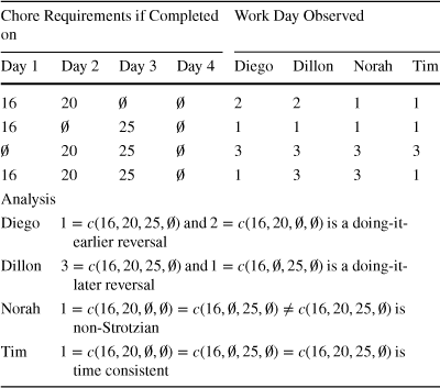
To illustrate how we use these definitions to analyze choices, Table 1 shows an example classification of four different completion functions (named Diego, Dillon, Norah, and Tim) within the choice quad derived from effort schedule
 .
.
We also test two common assumptions about completion functions, monotonicity and time invariance, that restrict choice across quads. Monotonicity requires that if
 ,
,
 , and
, and
 , then
 , with analogous requirements for all comparable two-date effort schedules. Time invariance requires that if an effort schedule is identical to another except that all effort requirements are shifted by one day, then the completion time also shifts by one day. For example, if
 and
and
 , then time invariance requires that
 if and only if
 .
.
Table 1 Classification of four completion functions within one quad
|
Chore Requirements if Completed on |
Work Day Observed |
||||||
|---|---|---|---|---|---|---|---|
|
Day 1 |
Day 2 |
Day 3 |
Day 4 |
Diego |
Dillon |
Norah |
Tim |
|
16 |
20 |
|
|
2 |
2 |
1 |
1 |
|
16 |
|
25 |
|
1 |
1 |
1 |
1 |
|
|
20 |
25 |
|
3 |
3 |
3 |
3 |
|
16 |
20 |
25 |
|
1 |
3 |
3 |
1 |
|
Analysis |
|||||||
|
Diego |
|
||||||
|
Dillon |
|
||||||
|
Norah |
|
||||||
|
Tim |
|
||||||


2 Experimental design
We design a real effort experiment to obtain data on participants’ task completion decisions and test sophistication, time consistency, and time invariance. Our four-day experiment presents each participant with two- and three-date effort schedules. Each participant makes “today” or “not today” decisions from effort schedules, which provide us with data on their completion function for each effort schedule. We selected effort schedules organized in quads to test time consistency and to use reversals to identify sophistication and naivete.
To observe a participant’s decisions in multiple different effort schedules we employ the random incentive system, providing incentive for a participant to report their true preferences of whether to work or not on each day. On the first day of the experiment, the participant is presented with all effort schedules for the experiment and is informed that one of these has been randomly chosen and will be implemented: the schedule-that-counts. The participant then must choose to complete chores “today” or “not today” for every effort schedule in which a
 option is available. If they choose “today” in the schedule-that-counts, then they complete the required number of extra chores today. Otherwise, when they log in the next day, they face a “today” or “not today” decision for those effort schedules with a non-trivial choice unless they previously chose “today” for that schedule.Footnote 5 This provides each participant with the incentive to make each decision as if it were the schedule-that-counts while allowing us to observe decisions from many effort schedules.
Our experiment presents each participant with effort schedules that are part of quads with completion options on either
 or
or
 . We construct effort profiles that specify the number of chores required to complete the task on each of the three consecutive available days. We selected effort profiles to be able to detect varying degrees of present and future bias; Table 3 displays the effort profiles we use. For each effort profile, the experiment includes quads of effort schedules with completion options on
 and
and
 .The latter effort schedules are obtained by shifting the former by one day, which enables us to test time invariance. We thus observe each participant make up to eight choices for one effort profile: one quad with opportunities to work on
 and one quad with options on
 . Some choices are censored when participants complete their extra chores early in their schedule-that-counts, but this design combined with the random incentive system ensures that each participant has at least a
 chance of making choices at
 .
.
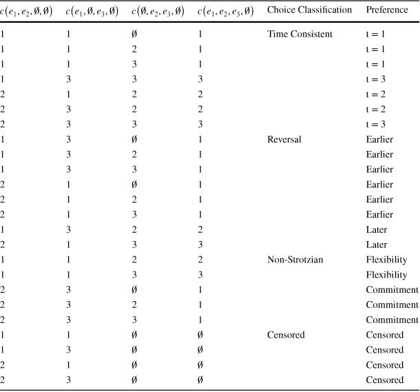
There are 24 possible combination of choices that a participant can make within a quad. We categorize each combination of choices as time consistent, a doing-it-earlier reversal, a doing-it-later reversal, non-Strotzian, or censored, as illustrated in Table 2. Seven of the 24 possible choice combinations can be rationalized by a time consistent completion function. Six possible choice combinations contain a doing-it-earlier reversal and two contain a doing-it-later reversal. These choice combinations are consistent with maximizing preferences in each period combined with, respectively, sophisticated and naive beliefs about future preferences. Five possible choice combinations are neither time consistent nor exhibit a reversal within a quad; we categorize these choice combinations as non-Strotzian. We further divide these into those in which the participant initially delays in
 , suggestive of a preference for flexibility, versus those in which the participant completes it immediately when facing
 , suggestive of a preference for commitment. We classify as censored four choice combinations in which the participant chooses to delay for
 and we do not observe
 choices, as censoring precludes a useful classification of such choices.
Table 2 Identification of all observable choice combinations within a quad
|
|
|
|
|
Choice Classification |
Preference |
|---|---|---|---|---|---|
|
1 |
1 |
|
1 |
Time Consistent |
t = 1 |
|
1 |
1 |
2 |
1 |
t = 1 |
|
|
1 |
1 |
3 |
1 |
t = 1 |
|
|
1 |
3 |
3 |
3 |
t = 3 |
|
|
2 |
1 |
2 |
2 |
t = 2 |
|
|
2 |
3 |
2 |
2 |
t = 2 |
|
|
2 |
3 |
3 |
3 |
t = 3 |
|
|
1 |
3 |
|
1 |
Reversal |
Earlier |
|
1 |
3 |
2 |
1 |
Earlier |
|
|
1 |
3 |
3 |
1 |
Earlier |
|
|
2 |
1 |
|
1 |
Earlier |
|
|
2 |
1 |
2 |
1 |
Earlier |
|
|
2 |
1 |
3 |
1 |
Earlier |
|
|
1 |
3 |
2 |
2 |
Later |
|
|
2 |
1 |
3 |
3 |
Later |
|
|
1 |
1 |
2 |
2 |
Non-Strotzian |
Flexibility |
|
1 |
1 |
3 |
3 |
Flexibility |
|
|
2 |
3 |
|
1 |
Commitment |
|
|
2 |
3 |
2 |
1 |
Commitment |
|
|
2 |
3 |
3 |
1 |
Commitment |
|
|
1 |
1 |
|
|
Censored |
Censored |
|
1 |
3 |
|
|
Censored |
|
|
2 |
1 |
|
|
Censored |
|
|
2 |
3 |
|
|
Censored |


The above table extends to quads derived from
 by adding 1 to every integer in the table, shifting all efforts and
 s in the header one position to the right while adding a
 in the first position of each effort schedule
Implementation We recruited 101 participants from the Simon Fraser University Experimental Economics Laboratory Research Participation System. Experiments were conducted entirely online. After signing up, each participant attended a live introductory Zoom session on a Friday. At the introductory session, an experimenter collected a consent form, read instructions aloud, and gave participants the opportunity to ask questions through a confidential chat. After answering all questions, participants were asked to demonstrate that they were able to sign-in to the online experiment interface using the university’s secure sign-in and complete one chore.Footnote 6 The experimenter provided technical support until all participants were successful. Each participant was paid $7 (CAD) for participating in the introductory session.
The experiment then took place the following Monday to Thursday. To complete the experiment, a participant was required to login to the experimental web interface on each of Monday, Tuesday, Wednesday, and Thursday. Each participant was sent a reminder email on each morning with a link to the experiment. After login, each participant was required to complete one mandatory chore each day. If a participant had not already completed extra chores, they were required to make task-completion decisions for all effort schedules where they had not previously made a “today” choice and there were two or more completion dates remaining. If a participant chose “today” in the schedule-that-counts (or if they had previously chosen “not today” for that schedule and the only remaining date to complete extra chores is the current date) they were required to complete the specified number of chores for that schedule to complete the task before the end of the day (23:59 Vancouver time). Each participant received an all-or-nothing payment of $25 for completing all experiment requirements beyond the introductory session. All payments were made by email transfer on the Sunday following the final experiment deadline.
Out of 101 participants who attended the online introduction and received the participation payment, 89 started the experiment on Monday, of which 82 completed all requirements over the four days. A breakdown of the exact experiment stage at which each participant dropped out is available in Online Supplement B. The remaining analyses focus only on the 82 participants who completed all requirements.
The baseline number of chores (20) and length of chore (40 characters) were chosen so the session would require less than one hour of a participant’s time over the four days to complete all chores and make all decisions required for the $25 completion pay. Our chore is the same a Greek character transcription used by Augenblick et al. (Reference Augenblick, Niederle and Sprenger2015); see Appendix Fig. 2 for a participant chore screen. A 40-character chore requires 40 button clicks with 100% accuracy. The median number of extra chores completed was 20.
Table 3 Experiment effort profiles

|
Effort |
Effort |
# Participants |
# Quads |
Versions |
|---|---|---|---|---|
|
Over Time |
Profile |
Observed |
Observed |
|
|
Increasing |
14, 20, 28 |
45 |
76 |
V1, V2 |
|
16, 20, 25 |
82 |
144 |
All |
|
|
18, 20, 22 |
82 |
144 |
All |
|
|
19, 20, 21 |
22 |
37 |
V2 |
|
|
Constant |
20, 20, 20 |
82 |
144 |
All |
|
Decreasing |
22, 20, 18 |
37 |
68 |
V3 |
|
25, 20, 16 |
37 |
68 |
V3 |
|
|
Total |
82 |
681 |
Each effort profile describes the number of chores required if working on Day 1, Day 2, or Day 3 (or for working on Day 2, Day 3, or Day 4)
We ran three versions of the experiment, varying the effort profiles participants faced across versions. In the first two versions of the experiment we used quads designed to have power to detect a participant’s present bias and their sophistication or naivete about said bias. For our third version, we included quads designed to test whether some participants exhibit a negative discount rate by choosing to exert more effort and complete the task at an earlier date. Specifically, we conducted Version 1 in a single session with 23 participants starting on July 20, 2020. After observing many “today” choices in Version 1, we added the (19, 20, 21) effort profile to Version 2 to allow us to detect even small degrees of present bias. Version 2 was conducted in a single session with 22 participants starting on July 27, 2020. Still observing many “today” choices, we chose effort profiles for Version 3 that enable us to detect whether participants would work today if doing so increased the number of chores required, which would indicate an opposing preference to those generated by discounting and present bias. We conducted Version 3 in two sessions, with 15 participants starting March 8, 2021 and with 22 participants starting March 29, 2021.
Table 3 displays the effort profiles participants faced in each version of the experiment. The effort profiles listed in Table 3 were used to form two quads, one quad with the effort schedule having availability at
 and a second quad with the same effort schedule shifted one day to
 .Footnote 7
Data Censoring We do not always observe two full choice quads from each effort schedule because the day on which a participant completes their extra chores is endogenous. When a participant completes their payoff-relevant extra chores at
 (Monday), they make no further task completion decisions. In these cases, we obtain no data for
 effort schedules nor do we obtain
 decisions from
 effort schedules. This partial censorship also occurs for
 effort schedules when the extra chores are completed at
 .
.
This endogenous censoring is inherent when studying any incentivized when-to-do-it choices. However, our design has a 1/2 probability that a
 schedule is the schedule-that-counts, and a 1/8 probability that a
 schedule with no option to do the extra chores on Monday is the schedule-that-counts. This design results in a 5/8 exogenous probability that a participant makes payoff relevant choices on at least two days. Our software randomly assigned 52 of 82 participants such an effort schedule, which we refer to as the non-endogenous subsample. We highlight this subsample when discussing results that otherwise could be subject to endogeneity. The remaining 30 participants generate data that is subject to endogenous censoring, including 5 participants who (endogenously) generate only censored quads.
Statistical Power We bootstrap likelihood-based confidence regions (Hall, Reference Hall1987) over simulated data to estimate our statistical power when restricting attention to the 52 participants in our non-endogenous subsample. We simulate data and check whether the observed proportion of participants who are time consistent, naive, and sophisticated falls within a 95% confidence region of the null proportion. Ex-post power analysis treats our observed data as the null and the confidence region around the null covers less than 7% of the parameter space. So we have 93% power to reject an alternative observation that is drawn randomly from a uniform distribution over the parameter space. In Online Supplement C we provide additional details on the ex-post confidence region and a complementary ex-ante power analysis.
3 Results
We designed our experiment to test sophisitication and naivete by observing choice reversals. However, we found a majority of participants displayed time consistency, primarily due to their tendency to complete the task as soon as possible. We begin by exploring this surprising result.
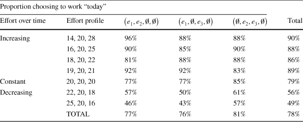
RESULT 1: Participants’ choices show an immediate completion tendency. In two-date effort schedules where waiting requires the same or less effort, 65% of participant choices are to work “today”.
Table 4 shows that over 75% of the individual choices from two-date effort schedules are choices to work “today”, including approximately half of two-date choices from the decreasing effort profiles (22, 20, 18) and (25, 20, 16).Footnote 8 Given the median participant required 75 s per chore, this implies a willingness to exert around 6 extra minutes of effort to complete the extra chores early.
Table 4 Proportion choosing to work “today” in two-date effort schedules (Non-endogenous subsample)
|
Proportion choosing to work “today” |
|||||
|---|---|---|---|---|---|
|
Effort over time |
Effort profile |
|
|
|
Total |
|
Increasing |
14, 20, 28 |
96% |
88% |
88% |
90% |
|
16, 20, 25 |
90% |
85% |
90% |
88% |
|
|
18, 20, 22 |
81% |
88% |
88% |
86% |
|
|
19, 20, 21 |
92% |
92% |
83% |
89% |
|
|
Constant |
20, 20, 20 |
77% |
77% |
85% |
79% |
|
Decreasing |
22, 20, 18 |
57% |
50% |
61% |
56% |
|
25, 20, 16 |
46% |
43% |
57% |
49% |
|
|
TOTAL |
77% |
76% |
81% |
78% |
|


65% of participant choices are to work “today” when combining constant and decreasing effort profiles
52% of participant choices are to work “today” when combining decreasing profiles
Next, we proceed to what we originally intended to be our main analysis by categorizing a participant’s choice quads into time consistent, doing-it-earlier reversal, doing-it-later reversal, or non-Strotzian, as shown inTable 2.
RESULT 2: Overall, choices in 82% of uncensored quads are time consistent. At the individual level, 50 of 82 participants are time consistent in all of their uncensored quads.
When all choice combinations over quads are considered regardless of censoring or endogeneity, 500 of 681 observations are time consistent. After removing the 83 censored observations, 498 of 598 (84%) uncensored choice combinations are time consistent, 397 of which exhibit a consistent preference to complete the extra chores on the first available day. Table 5 provides the classifications by effort profile and remarkably within every effort profile, over two-thirds (66%) of all participant choice quads are time consistent; the level or interest rate on effort does not appear to affect overall rates of time consistency.Footnote 9 Among the time inconsistent choice combinations, we observe similar rates of reversals and non-Strotzian observations (9% and 6% of “TOTAL” observations in Table 5). If choice data were generated randomly by independently mixing at each choice (“RANDOM” in Table 5), 33% of choice combinations would be time consistent, and 35% would exhibit a reversal.
Table 5 Classifying choice combinations within a quad by effort profile (all data)

|
Effort |
Time Consistent |
Reversal |
Non- |
Censored |
Quads |
|||
|---|---|---|---|---|---|---|---|---|
|
Profile |
1st day |
2nd day |
3rd day |
earlier |
later |
Strotz |
Observed |
|
|
14, 20, 28 |
72% |
3% |
7% |
4% |
3% |
7% |
5% |
76 |
|
16, 20, 25 |
69% |
2% |
6% |
8% |
1% |
3% |
10% |
144 |
|
18, 20, 22 |
65% |
4% |
5% |
8% |
1% |
7% |
11% |
144 |
|
19, 20, 21 |
65% |
5% |
5% |
5% |
3% |
5% |
11% |
37 |
|
20, 20, 20 |
51% |
6% |
8% |
10% |
1% |
7% |
16% |
144 |
|
22, 20, 18 |
37% |
7% |
24% |
7% |
0% |
9% |
16% |
68 |
|
25, 20, 16 |
38% |
7% |
26% |
10% |
0% |
3% |
15% |
68 |
|
TOTAL |
58% |
5% |
10% |
8% |
1% |
6% |
12% |
681 |
|
uncensored |
66% |
5% |
12% |
9% |
1% |
2% |
598 |
|
|
RANDOM |
13% |
10% |
10% |
25% |
10% |
23% |
9% |
|
|
uncensored |
14% |
11% |
11% |
28% |
11% |
25% |
||
RANDOM is the expected proportion if all choices are random and independent
“1st day” is
 in
in
 effort schedules and
 in
in
 effort schedules
Table 6 Classifying choice combinations within a quad by effort profile (non-endogenous subsample)

|
Effort |
Time Consistent |
Reversal |
Non- |
Censored |
Quads |
|||
|---|---|---|---|---|---|---|---|---|
|
Profile |
1st day |
2nd day |
3rd day |
earlier |
later |
Strotz |
Observed |
|
|
14, 20, 28 |
79% |
4% |
0% |
4% |
4% |
8% |
0% |
24 |
|
16, 20, 25 |
75% |
2% |
6% |
12% |
0% |
6% |
0% |
52 |
|
18, 20, 22 |
73% |
4% |
4% |
10% |
2% |
8% |
0% |
52 |
|
19, 20, 21 |
75% |
0% |
0% |
8% |
8% |
8% |
0% |
12 |
|
20, 20, 20 |
60% |
10% |
2% |
12% |
4% |
13% |
0% |
52 |
|
22, 20, 18 |
36% |
14% |
29% |
4% |
0% |
18% |
0% |
28 |
|
25, 20, 16 |
32% |
14% |
36% |
14% |
0% |
4% |
0% |
28 |
|
TOTAL |
63% |
7% |
10% |
10% |
2% |
9% |
248 |
|
This table only uses only the
 effort schedules, and only the 52 participants whose randomly assigned schedule-that-counts does not include

The full set of data in Table 5 are subject to endogenous sampling and censoring. Table 6 displays results for the non-endogenous subsample, and further drops the choice combinations over quads derived from
 effort schedules since they are subject to endogenous observation of choices at
 (Wednesday). The data in Table 6 have zero censored observations by construction, yet still exhibit a very similar mix of choice combinations to the “Total uncensored” data from Table 5.
Within the non-endogenous subsample, 28 of 52 participants are time consistent in 100% of observed choice combinations, and 18 of these 28 chose to work “today” in every choice. Since we observe this subsample make choices on at least two days, all of these tests of time consistency are non-trivial. All remaining tables in the main text of results include only this non-endogenous subsample – though the similar values in Tables 5 and 6 suggest that data censoring does not appear to drive our results on time consistency.
The remaining 30 of 82 participants were randomly assigned a schedule-that-counts which allowed them to complete their extra chores on Monday, and this subsample is subject to endogenous selection. The participants in this set who chose to work “today” for their schedule-that-counts do not make any more decisions after Monday.Footnote 10 We find that 17 of these participants exclusively generate choice combinations that are time consistent, and another 5 only generate censored choice combinations, and thus satisfy time consistency trivially. The remaining 8 of these participants generated at least one reversal or non-Strotzian choice combination.
Time consistency is tested using a choice combination over a single quad, but an additional consideration is whether a participant’s choices are collectively sensible when looking across quads.
RESULT 3: Overall, fewer than 5% of observations need to be dropped to make every participant consistent with monotonicity. Among the participants who are time consistent within every quad, 90% also demonstrate monotonicity across all quads.
Monotonicity links preferences across effort values and requires participants to consistently prefer exerting less effort while controlling for completion time. We evaluate whether a participant violates monotonicity, considering every two-date choice across all quads in the experiment.
We count the total number of monotonicity violations for each participant. We find that 58 of 82 participants (71%) demonstrate no violations of monotonicity in their choice data. Of the 50 participants who were time consistent in 100% of their classified choice combinations, only 5 made a choice violating monotonicity, thus 45 of 82 participants were both time consistent and monotonic in all choices.
For those participants who do violate monotonicity, we use the Houtman-Maks Index (HMI) to represent the maximal proportion of data which can be collectively consistent with monotonicity (Houtman and Maks, Reference Houtman and Maks1985; Heufer and Hjertstrand, Reference Heufer and Hjertstrand2015; Demuynck and Hjertstrand, Reference Demuynck, Hjertstrand, Anderson, Richard and Barnett2019). This involves a simple linear optimization for each participant, minimizing the number of observations removed, subject to the constraint that there are zero monotonicity violations in the remaining dataset. In total, 76 of 1726 observations are removed for a weighted mean HMI of 0.955, and the mean HMI among those with at least one violation is 0.86. The distribution of HMI by participant in Fig. 1 further demonstrates that monotonicity violations are rare and concentrated in a minority of individuals.

Fig. 1 Participant Houtman-Maks index - monotonicity
When the same effort tradeoff is observed on different days, a participant who makes a different “today” or “not today” choice has violated time invariance. A violation of time invariance could suggest an unobserved preference to complete the task on a specific day.
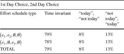
RESULT 4: Time invariance is satisfied in 79% of comparable decision pairs.
Time invariance requires us to compare a participant’s choices in
 quads to their analogous choices in
 quads. Restricting attention to binary choices from the non-endogenous subsample, there are 496 total possible tests of time invariance.Footnote 11 Time invariance is satisfied in 79% of tests, and 23 of 52 participants in the non-endogenous subsample satisfy time invariance in every test.
Table 7 displays the proportion of two-date choices that violate time invariance when we observe a participant make choices from comparable effort schedules on two different days. The relative scarcity of violations of time invariance suggest specific day-of-the-week preferences are driving choices in at most 22% of tests. The number of chores and the interest rate on effort do not appear to systematically affect the rate of failure of time invariance across schedules (Appendix Table 10).
Table 7 Time invariance violations by choice set (non-endogenous subsample)
|
1st Day Choice, 2nd Day Choice |
|||
|---|---|---|---|
|
Effort schedule type |
Time invariant |
“today”, “not today” |
“not today”, “today” |
|
|
79% |
8% |
13% |
|
|
78% |
8% |
13% |
|
TOTAL |
79% |
8% |
13% |


The small response to a negative interest rate on effort apparent in Table 6 indicates that choices are not well represented by a standard model of intertemporal preferences in which participants discount costly future relative to immediate effort. We conduct a structural estimation to facilitate a comparison of behavior in our experiment to existing work.
RESULT 5: Structural estimation of a model of quasi-hyperbolic discounting yields
 , capturing a strong tendency to complete real effort tasks immediately.
We model the probability of choosing “today” as resulting from a latent utility model. Consider only the two-date decisions, and let
 denote the effort requirements for periods t and
 . Let
. Let
 denote a “today” choice at t and
 denote a “not today” choice. We assume that
 , where
 represents the time-t (unobserved) utility difference between choosing “today” and “not today”. We specify a structural quasi-hyperbolic discounting model with a linear disutility-of-effort:
 =
=
 where
where
 and
and
 with
with
 and
and
 scalar time preference parameters to be estimated.
The net utility of working “today” can be written as
 . We assume there is some variation in individual values of
 due to individual preference shocks, and specify a logit regression
 , where
 and
and
 a standard binary logit model with no intercept term.Footnote 12 We recover estimates of
 and use them to estimate
 ;
;
 ; and
; and
 .Footnote 13 We cluster standard errors by participant, and recover asymptotic standard errors for the parameter estimates using the delta method. Parameter estimates and their asymptotic standard errors are presented in Table 8. We provide the underlying logit regression estimates of
 and further details in Appendix Tables 11, 12, and 13.
Table 8 Results of structural logit estimation (non-endogenous subsample)

|
Parameter |
Estimate (Std. Error) |
Confidence Intervals (
|
|
|---|---|---|---|
|
Lower Bound |
Upper Bound |
||
|
Present Bias
|
1.54 |
1.11 |
1.96 |
|
(0.22) |
|||
|
Discount Factor
|
0.93 |
0.83 |
1.03 |
|
(0.050) |
|||
|
Disutility of Effort
|
0.14 |
0.06 |
0.22 |
|
(0.042) |
|||
|
Observations |
743 |
||
|
Clusters |
52 |
||


Estimated using binary effort schedules only. Standard errors of logit regression are clustered by individual participant. Asymptotic standard errors estimated using the delta method (derivation in Appendix)
Previous studies of intertemporal preference consistently estimate values of
 , with the interpretation being that there is additional (non-geometric) discounting of all future periods relative to the present. Two recent meta analyses have found mean values of
 that are significantly less than one when conditioning on studies that used real-effort tasks (Imai et al., Reference Imai, Rutter and Camerer2020) find an average
 of 0.88 across 9 studies) or non-monetary rewards (Cheung et al., Reference Cheung, Tymula and Wang2021) find an average
 of 0.66 across 5 studies). Imai et al. (Reference Imai, Rutter and Camerer2020, Table 8) estimate that each of the main features of our experiment – non-monetary reward, conducted online, and ‘immediate: by end of day’ (as opposed to a longer time frame for immediate costs and rewards) – have a negative or insignificant effect on the value of
 . Imai et al. (Reference Imai, Rutter and Camerer2020, p. 1804) demonstrate that the standard error of the
 estimate is negatively correlated with the value of the
 estimate in published real effort studies, “suggesting the existence of modest selective reporting in the direction of over-reporting
 in studies using a real-effort task.”
The participants in this experiment had a clear disposition to complete the extra chores “today”, and this is reflected in the estimate of
 , as caring more about future utility than today’s utility would result in the observed participant disposition to complete the task today (with 580 of 743 two-date choices to work “today”). The estimated value of the disutility of effort parameter has the expected sign. Geometric discounting is identified from the difference in choices when the delay is
 days versus
 , but does not appear to be a significant driver of choice since
 . However, the strong tendency to immediately complete the task immediately makes it difficult to precisely estimate
 and
and
 since any combination of
 can drive such a tendency, and our estimates of both
 and
and
 are imprecise.
The difference between our results and the results from previous real effort experiments studying time preferences warrants further discussion. We next discuss six classes behavioral explanations for our findings.Footnote 14 We compare the ability of each to fit both our data and the stylized findings of prior real effort experiments that found evidence of present bias in a CTB experiment (Augenblick et al., Reference Augenblick, Niederle and Sprenger2015).
4 Discussion: explaining an immediate completion tendency
Our experiment is designed to measure a person’s sophistication or naivete about their own time inconsistency. Yet we discovered far more time consistency than we expected based on prior work from economics experiments (e.g. Thaler Reference Thaler1981; Read & Van Leeuwen Reference Read and Van Leeuwen1998; Ashraf et al. Reference Ashraf, Karlan and Yin2006), including other experiments that use designs with similar real effort tasks (Augenblick et al., Reference Augenblick, Niederle and Sprenger2015; Augenblick & Rabin, Reference Augenblick and Rabin2019; Augenblick, Reference Augenblick2018)). This appears to be driven by a strong tendency to complete tasks immediately – even when this requires additional effort. We estimate a structural model to compare our results to previous work and we find paramater values that imply our participants have future-biased preferences. While some previous studies using monetary or hypothetical rewards have found evidence of future bias (e.g. Sayman & Öncüler Reference Sayman and Öncüler2009; Attema et al. Reference Attema, Bleichrodt, Rohde and Wakker2010; Takeuchi Reference Takeuchi2011; Montiel Olea & Strzalecki Reference Olea, Luis and Strzalecki2014; Aycinena et al. Reference Aycinena, Blazsek, Rentschler and Sandoval2019, Reference Aycinena, Blazsek, Rentschler and Sprenger2022), recent meta-analyses document that such a finding is the exception and not the norm, and has no published precedent in real effort tasks (Imai et al., Reference Imai, Rutter and Camerer2020; Cheung et al., Reference Cheung, Tymula and Wang2021).
Next we outline six decision models that can rationalize an early completion tendency and discuss their consistency with both our data and related experiments. For the purpose of this Discussion section, we take Augenblick et al. (Reference Augenblick, Niederle and Sprenger2015) as a typical intertemporal choice experiment that uses real effort tasks and finds a preference to delay work and we evaluate alternative theoretical explanations against both our findings and theirs. Because we use their Greek transcription task and we both use student participants, there seem to be few economically-important differences in our designs that could explain why our participants seem to make qualitatively different trade-offs between earlier versus later effort. The one economically crucial difference between the designs is that our participants make decisions once-and-for-all, while Augenblick et al. participants make effort allocations at-the-margin: each of their decisions has a participant allocate required chores between an earlier and a later date along a continuous convex time budget (CTB).
Quasi-hyperbolic discounting We find quasi-hyperbolic discounting an unsatisfactory explanation for our findings. To rationalize the early completion tendency in our data with a structual model of quasi-hyperbolic discounting requires
 , which corresponds to a future bias. In contrast, past applications are motivated by present bias (
 , Laibson (Reference Laibson1997), O’Donoghue and Rabin (Reference O’Donoghue and Rabin1999)) and published experimental studies using real effort tasks have found evidence of present bias (Imai et al., Reference Imai, Rutter and Camerer2020; Cheung et al., Reference Cheung, Tymula and Wang2021). Our results thus present a puzzle relative to experiments that study intertemporal allocations involving real effort tasks that have been taken as evidence for present bias.Footnote 15
One difference between our study and most existing literature that use real effort experiments to study intertemporal choice is that we use delays on the order of 1–2 days, whereas most existing work studies longer delays. However, Augenblick (Reference Augenblick2018) studies discounting in the same real effort task over delays as short as two hours and finds that two-thirds of discounting that occurs within one week occurs in the first day. We thus rule out our 1–2 day delay length as a possible explanation for the future bias we find.
Anticipatory utility Dread from anticipating the need to complete real effort tasks in the future can generate an immediate completion tendency, but could also lead to a bias to complete more chores earlier in CTB designs, making it unclear whether anticipatory utility is a satisfactory explanation for our results. In Online Supplement A, we modify Loewenstein’s (Reference Loewenstein1987) model of anticipatory utility to allow for present bias and study its relation to our experimental design and CTB designs. We show that the parameter restrictions required to explain an immediate completion tendency in our experiment also implies future bias in a CTB design, the opposite of what Augenblick et al. (Reference Augenblick, Niederle and Sprenger2015) and similar papers observe. This calls into question whether anticipatory utility is the right explanation for our findings.
More general models of anticipatory utility beyond Loewenstein’s may be more successful. Anticipatory utility will tend to lead people to postpone good things and speed up bad things – acting against standard discounting and present bias. But if loss aversion creates a stronger motive for real effort tasks than for receipt of good things, then anticipatory utility may be particularly relevant in our environment (Hardisty & Weber, Reference Hardisty and Weber2020). However, this motive would apply in all real effort designs, not just ours. Thus it does not seem like an obvious approach to jointly explain our finding and present bias in CTB designs. One possibility is that anticipatory utility displays diminishing sensitivity to the quantity of effort in ways that are inconsistent with Loewenstein’s model. In the most extreme version of this, anticipatory utility would act like a fixed cost of having to complete the task in the future – like a a fixed cost of delay, which we discuss below.
Decision costs We rule out decision costs as an explanation for the early completion tendency we find. A participant who experiences a subjective cost of making each choice and fully integrates the random incentive scheme might be biased, relative to their underlying time preferences, to choose “today” in our experiment because this reduces their probability of having to make choices tomorrow and thereby avoids any future subjective decision costs. We find this explanation implausible in our setting for three reasons. First, our instructions and comprehension tests (while clear and complete) did not emphasize this relatively subtle aspect of the design. Second, a long experimental literature has tested whether people tend to make each choice in isolation or rationally account for the experiment’s incentive scheme – and this work has almost universally found that most people make each choice in isolation (Starmer & Sugden, Reference Starmer and Sugden1991; Cubitt et al., Reference Cubitt, Starmer and Sugden1998; Hey & Lee, Reference Hey and Lee2005; Freeman & Mayraz, Reference Freeman and Mayraz2019). Third, this explanation should be more powerful on Monday than Tuesday: completing the task on Monday avoids 19 Tuesday choices (plus possibly avoids Wednesday choices), whereas completing the task on Tuesday avoids only 9 Wednesday choices. However, we see roughly the same degree of early completion bias in Monday and Tuesday choices: in Table 4 we see 77% early completion over
 schedules when 19 decisions could be avoided, but 81% early completion over
 schedules when only 9 decisions could be avoided. For the effort profile (20, 20, 20), we see that early completion occurs in 77% of opportunities when 19 decisions could be avoided, but early completion occurs in 85% of cases for when only 9 decisions could be avoided. Our participants showed a stronger early completion tendency when the number of future decisions was lower, and this strongly suggests that a motive to avoid facing future decisions is not a good explanation of the early completion tendency we find.
Cost of keeping track Both our experiment and Augenblick et al. (Reference Augenblick, Niederle and Sprenger2015) require subjects to log on and complete a minimal number of chores in all periods regardless of choices, and provide sign-in reminders to subjects. This makes an anticipation of a cost of keeping track Haushofer (Reference Haushofer2015) or of memory limitations Ericson (Reference Ericson2017) not particularly compelling explanations for our finding.
Fixed cost of delay Hardisty et al. (Reference Hardisty, Appelt and Weber2013) present a model in which a person makes intertemporal choices as if they experience a fixed cost of delay; a particular interpretation of this model might explain our findings, but we have some caveats. For receipt of goods, this model will result in behavior that looks like present bias. But for bads – like our real effort tasks – it could result in an immediate completion tendency over low stakes in spite of a preference for delay over high stakes.Footnote 16
One possible weakness of this explanation is that both our design and Augenblick et al. (Reference Augenblick, Niederle and Sprenger2015) require a login and mandatory chores in all periods. If accounted for by participants, all participants should experience both real and subjective fixed costs each period regardless of their choices. Thus any fixed costs of delay should not influence behavior in either of our experiments. However, Ellis and Freeman (Reference Ellis and Freeman2021) show that most people are well-described as narrow bracketers in a variety of domains. In our setting, a narrow bracketer only responds to the choice in front of them, and ignores the mandatory logins and chores when making each choice. We thus consider whether a fixed cost of delay combined with narrow bracketing can explain our results.
A person who experiences a subjective fixed cost of delay and brackets narrowly should exhibit an early completion tendency in our design. When subjective fixed costs are sufficiently large, they should also exhibit an early completion tendency in CTB designs whenever the stakes are sufficiently low for it to be worthwhile to complete all required chores immediately to avoid fixed costs. But conditional on making interior allocations in a CTB design fixed costs should not influence trade-offs, and thus if people are present biased after controlling for subjective fixed costs the CTB will only detect present bias and not subjective fixed costs.Footnote 17 Thus, the combination of narrow bracketing and fixed cost discounting can perhaps accommodate both the early completion tendency we find and present-biased choices in the Augenblick et al. (Reference Augenblick, Niederle and Sprenger2015) CTB design.
Get-it-started bias A bias to get tasks started can possibly explain our finding. Using a very different type of real effort task Rosenbaum et al. (Reference Rosenbaum, Gong and Potts2014) and Fournier et al. (Reference Fournier, Stubblefield, Dyre and Rosenbaum2019a; Reference Fournier, Coder, Kogan, Raghunath, Taddese and Rosenbaumb) document a bias to get tasks started. In our design, starting and finishing a task are tied, so a get-it-started bias would lead to an early completion tendency in our experiment. In a CTB, starting and finishing a task are de-coupled, so a participant can satisfy their get-it-started bias but still allocate effort to the future. If participants also exhibit present bias, a CTB design should detect this. Thus a get-it-started bias is potentially consistent with both our finding and the findings of Augenblick et al. (Reference Augenblick, Niederle and Sprenger2015). We consider this the most plausible explanation for behavior in our experiment.
Future research Our findings present a challenge to the standard model of intertemporal choice, quasi-hyperbolic discounting, on a domain where previous literature suggests it ought to apply. Our findings also challenge existing models of anticipatory utility, although more general models of anticipatory utility might be more successful. We find a get-it-started bias to be a plausible though somewhat unsatisfying explanation, in part because it is far from standard models of intertemporal choice considered in the behavioral economics literature. Hardisty & Weber (Reference Hardisty and Weber2020, Experiment 3) find that participants are more prone to immediately eat bad-flavored jelly beans than good flavored jelly beans, and they link to anticipatory utility without providing any formal modeling. A carefully designed incentivized experiment could shed further light on why in some choices (like those in our experiment) participants exhibit an early completion tendency whereas in others they tend to delay. Further work is needed to understand whether more general models of anticipatory utility or discounting can provide a reasonable account of intertemporal decisions involving real-effort tasks.
We also explored two other standard properties assumed in most models of intertemporal choice—time invariance and monotonicity—and we do not detect systematic failures of either property. This suggests that these are both descriptively reasonable properties to retain.
Appendix
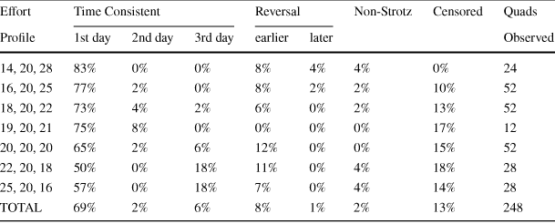
Table 9 Classifying choice combinations within a quad by effort profile (non-endougenous subsample)
|
Effort |
Time Consistent |
Reversal |
Non-Strotz |
Censored |
Quads |
|||
|---|---|---|---|---|---|---|---|---|
|
Profile |
1st day |
2nd day |
3rd day |
earlier |
later |
Observed |
||
|
14, 20, 28 |
83% |
0% |
0% |
8% |
4% |
4% |
0% |
24 |
|
16, 20, 25 |
77% |
2% |
0% |
8% |
2% |
2% |
10% |
52 |
|
18, 20, 22 |
73% |
4% |
2% |
6% |
0% |
2% |
13% |
52 |
|
19, 20, 21 |
75% |
8% |
0% |
0% |
0% |
0% |
17% |
12 |
|
20, 20, 20 |
65% |
2% |
6% |
12% |
0% |
0% |
15% |
52 |
|
22, 20, 18 |
50% |
0% |
18% |
11% |
0% |
4% |
18% |
28 |
|
25, 20, 16 |
57% |
0% |
18% |
7% |
0% |
4% |
14% |
28 |
|
TOTAL |
69% |
2% |
6% |
8% |
1% |
2% |
13% |
248 |
This table only uses only the
 effort schedules, and only the 52 participants whose randomly assigned choice that counts does not include

Table 10 Time invariance by effort schedule (non-endogenous subsample)

|
Effort Profile |
First Day Choice, Second Day Choice |
||
|---|---|---|---|
|
Time Invariant |
“today”, “not today” |
“not today”, “today” |
|
|
14, 20, 28 |
90% |
4% |
6% |
|
16, 20, 25 |
87% |
7% |
7% |
|
18, 20, 22 |
80% |
9% |
12% |
|
19, 20, 21 |
83% |
8% |
8% |
|
20, 20, 20 |
70% |
12% |
17% |
|
22, 20, 18 |
70% |
11% |
20% |
|
25, 20, 16 |
75% |
2% |
23% |
|
Grand Total |
79% |
8% |
13% |
Table 11 Structural logit estimates (non-endogenous subsample)

|
Dependent variable: |
|
|---|---|
|
Today1 |
|
|
EffortToday |
−0.140
|
|
(0.042) |
|
|
EffortNotTodayK1 |
0.199
|
|
(0.041) |
|
|
EffortNotTodayK2 |
0.185
|
|
(0.043) |
|
|
Observations |
743 |
|
Log Likelihood |
−358.575 |
|
Akaike Inf. Crit |
723.150 |


 p<0.1;
 p<0.05;
 p<0.01
Table 12 Variance-covariance matrix of structural logit estimates (Non-endogenous subsample)

|
EffortToday |
EffortNotTodayK1 |
EffortNotTodayK2 |
|
|---|---|---|---|
|
EffortToday |
0.001803 |
|
|
|
EffortNotTodayK1 |
|
0.001716 |
0.001725 |
|
EffortNotTodayK2 |
|
0.001725 |
0.001826 |


Table 13 Variance-Covariance Matrix of Parameter Estimates using Delta Method

|
CRow1 |
CRow2 |
CRow3 |
|
|---|---|---|---|
|
CRow1 |
0.046933 |
|
0.007851 |
|
CRow2 |
|
0.002545 |
|
|
CRow3 |
0.007851 |
|
0.001803 |


Deriving parameter estimates and variance-covariance matrix for delta method
We estimate the logistic regression:

For our structural model, we are interested in the values of

 ),
),
 (
(
 ), and
 (
(
 )
)
If
 then the distribution of f(b) is
 where
where
 .
.
Let
 . Then,
 .
.
The estimated variance matrix of interest is
 See Figs. 2, 3.
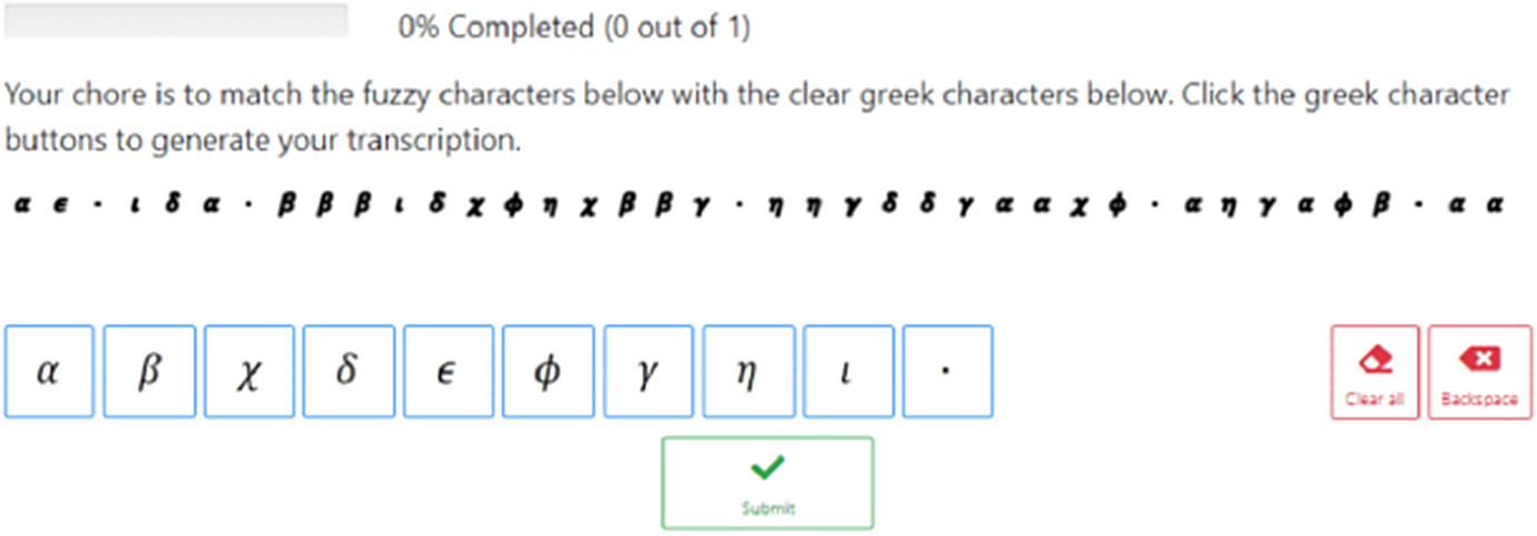
Fig. 2 Experiment chore The status at the top of this figure implies this is the chore screen on a day when a participant has chosen to only complete the minimum of one chore
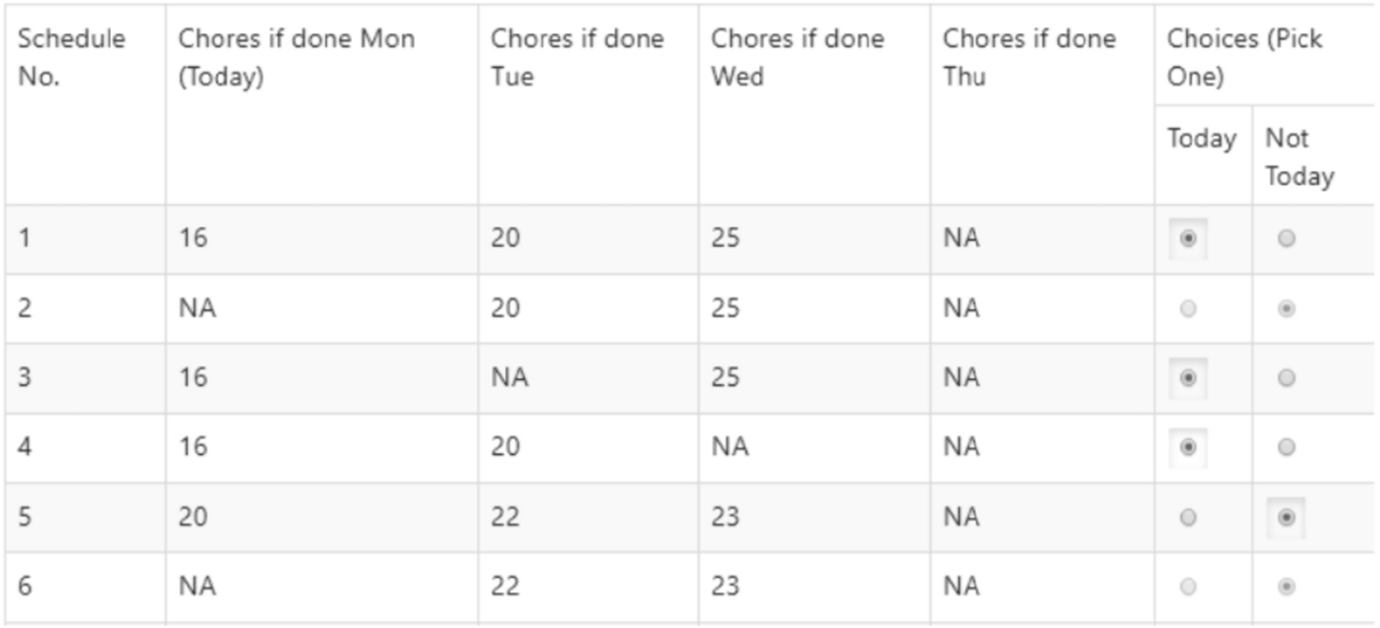
Fig. 3 Excerpt of experiment decision table (Monday) Effort schedules like Schedule No. 2 and Schedule No. 6 are displayed to participants so they are aware of all possible schedules-that-count, but the buttons are fixed on “Not Today” for these schedules because they are Not Available (NA) to be completed on Monday
Supplementary Information
The online version contains supplementary material available at https://doi.org/10.1007/s10683-024-09824-2.
Acknowledgements
We thank Victor Aguiar, Priscilla Fisher, Henry Schneider, and conference participants at the World ESA 2022 for feedback that improved our paper. This research was funded by SSHRC IDG 430-2016-00193 and conducted under SFU REB certificate #20160245. Replication and supplementary material for the study is available at https://osf.io/XBACF/.


 Open access