2.1. Problem formulation

The problem at hand involves the determination of the pedestrian-level flow field, framed as an image-to-image translation task. Specifically, the task is approached by leveraging a set of preprocessed geometries denoted as $ X $ , represented as grey-scale images. These images are input into a model $ f $ with the objective of learning a mapping to a pre-computed flow field $ Y $ , derived from a RANS simulation. Each pixel value in an individual image $ {x}_i\in X $ encodes the heights of the buildings within the spatial domain. In contrast, the corresponding output image $ {y}_i $ is a 3-channel RGB image, where each channel represents the $ x,y,z $ velocity components at a 2 m height. It is crucial to note that the boundary conditions for the CFD solutions are uniform across all data points in $ Y $ and are implicitly incorporated into the model. The learning process, encapsulated in the mapping from $ X\to Y $ , is achieved by adjusting the model’s free parameters denoted as $ \theta $ . This adjustment is facilitated through backpropagation, employing a defined set of loss function equations:

(1) $$ {f}_{\theta }:{x}_i\to {y}_i\hskip1em {x}_i,{y}_i\in X,Y $$

(2) $$ {\mathit{\min}}_{\theta}\left[\frac{1}{2}\left(\parallel {y}_i-f\left(x,\theta \right){\parallel}_1+\parallel {\hat{y}}_i-f\Big(\hat{x},\theta \Big){\parallel}_1\right)\right] $$

The loss function employed in this study aims to quantify the disparity between the model’s output and the precomputed flow fields, utilising the mean absolute error (MAE). To further emphasise the significance of the central section in the evaluation process, an additional term has been introduced. This supplementary term accounts for the central portion of the image, $ \hat{x} $ , acknowledging its heightened importance in capturing nuanced details critical to the accuracy of the flow field prediction. The loss function is designed as the average of two components: the MAE computed across the entire image and the MAE calculated for a cropped central section. This approach ensures a balanced evaluation, promoting both overall accuracy and the model’s ability to capture fine details in the central region of the flow field.

2.2. Geometries

The training dataset used in this study consists of 163 distinct synthetic geometries, each serving as the foundation for generating eight individual CFD scenarios. These scenarios account for wind flow from each of the cardinal and ordinal directions. The choice of a circular formation for each geometry introduces a deliberate uniformity among simulations, particularly in terms of wind interaction around the outer edge of the urban configuration.

The buildings within each geometry are characterised by simple, smooth prisms, featuring either sharp corners or fillet angles reminiscent of architectural styles found in early-stage design. Each building maintains a consistent cross-sectional area along its height axis. Notably, the architectural design intentionally omits intricate features such as bridges, skywalks, balconies, or masts. Moreover, it is crucial to highlight that the buildings in the synthetic geometries are entirely impermeable, contributing to a simplified yet representative simulation environment. Each geometry within the dataset exhibits variability in terms of density, building height, and the extent of open areas, providing a diverse range of scenarios for training the model.

2.3. CFD simulations

The CFD solutions in this study were generated using the open-source OpenFOAM v2206 software, utilising the simpleFOAM steady-state solver tailored for incompressible turbulent flow. To model turbulence closure, a $ k-\unicode{x025B} $ model was employed, with specific coefficients, $ {C}_{\mu },{C}_{\unicode{x025B} 1},{C}_{\unicode{x025B} 2},{\sigma}_k $ set to $ \mathrm{0.09,1.44,1.92,1.11} $ , respectively, as per the work of Hargreaves et al (Hargreaves and Wright, Reference Hargreaves and Wright2007).

The synthetic geometries were positioned at the centre of a cylindrical domain with a diameter of 3000 m and a height of 300 m. An internal orthogonal grid was used to refine the mesh within 75 m from the extremities of the geometry. This refinement not only enhanced cell quality but also provided a higher spatial resolution crucial for capturing the nuanced physics of the flow. The mesh resolution was adaptively adjusted, progressively increasing cell volumes with distance from the ground where a finer resolution was deemed unnecessary, thereby mitigating computational load. The mesh generation around the building geometries was facilitated by the in-built snappyHexMesh routine (OpenFOAM, n.d.).

The inflow conditions were characterised by a logarithmic profile with a reference velocity of 5 m/s at a height of 10 m. A slip boundary condition was applied at the top surface of the domain. A total of 1304 unique results were obtained by simulating wind flow from eight directions for each geometry, considering both cardinal and ordinal directions. The solver was run for 1000 iterations with a time step size $ \Delta t $ of 1 s chosen as a tradeoff between accuracy, convergence, and computational efficiency to generate a sufficiently robust training dataset.

2.4. Data preparation

For each of the 163 unique geometries, a transformation into a 2-dimensional grey-scale image is performed using the PyVista Python package (Bane Sullivan and Alexander Kaszynski, Reference Bane and Alexander2019), yielding images with dimensions $ H\times W=1024\times 1024 px $ . Each pixel represents an area of approximately 1 m² and has a value within the range of $ \left[0,1\right] $ representing the scaled height of the building at that specific point in space.

Similarly, the precomputed flow fields undergo preparation also using the PyVista package. a slice of the $ XY $ plane is taken, capturing the velocity components of the flow field in separate channels as RGB pixel values. Specifically, the red, green, and blue channels encode the $ x,y,z $ velocity components, resulting in a tensor of size $ H\times W\times C=1024\times 1024\times 3px $ . 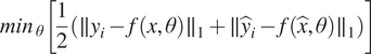A colour mapping is applied to the velocity components, with $ \left[-6,6\right]\to \left[0,1\right] $ for $ x,y $ direction and $ \left[-2,2\right]\to \left[0,1\right] $ for the $ z $ component. A sample training pair is shown in Figure 1.

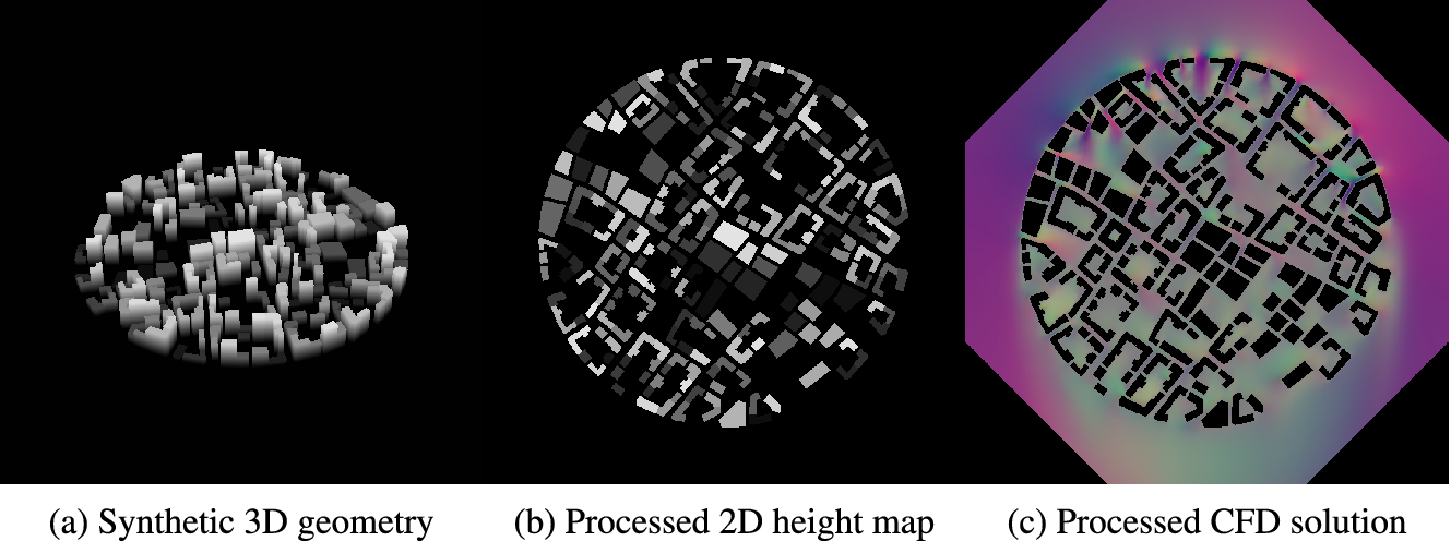
Figure 1. Training Data Overview: (a) 3D model of a synthetic geometry used to generate training data for the deep learning model. (b) Processed geometry, a 2D representation of the synthetic geometry after preprocessing, where pixel colour corresponds to the height of the buildings. (c) Postprocessed CFD Data where the RGB channels encode the velocity components in the x, y, and z directions. This image provides a visual representation of the ground truth used for training and evaluating the deep learning model.

To ensure consistency, each of the 1304 image representations of the velocity fields is rotated such that the wind inflow is from the top of the image. The relevant components are transformed using a rotation matrix congruent with their shift in the frame of reference. Augmentation is further applied by mirroring each rotational orientation about the Y-axis, resulting in the full 16 octagonal symmetries for each geometry. Consequently, the final training set comprises 2608 geometry-flow field pairs, providing a robust and diverse dataset for model training. To describe the velocity flow field in our analysis, we employ a Cartesian coordinate system with axes $ {U}_x $ , $ {U}_y $ , and $ {U}_z $ , representing the horizontal, vertical and depth components. Positive values indicate motion toward the right and top of the image for the $ {U}_x $ and $ {U}_y $ components and emerging from the page for the $ {U}_Z $ component.

Given that the geometries undergo rotations at angles such as 45, 135, 225 degrees, etc., a notable consequence is the absence of data in the corners of the resulting images. While such data gaps do not pose an issue when rotations occur in multiples of 90 degrees, the irregular angles necessitate a corrective measure. To address this, a corner mask is systematically applied to all images. This mask effectively removes the data in the corners, ensuring uniformity across all orientations and mitigating confusion in the model, thereby enhancing the overall consistency and reliability of the dataset.

2.5. Model architecture

The model architecture draws inspiration from the image-to-image multilayer perceptron (MLP) mixer model introduced by Mansour et al. (Mansour et al., Reference Mansour, Lin and Heckel2023). This supervised learning model, comprising solely of linear transformations, nonlinear activations, and data transpositions, demonstrated state-of-the-art performance in computer vision tasks such as reconstructing noisy images. Information transfer in this architecture is facilitated through MLP layers acting on linear transformations of input images across all spatial dimensions and token channels. Unlike a convolutional neural network, which inherently captures local spatial relationships due to their convolutional nature and receptive fields, giving them a strong inductive bias toward translation invariance while allowing them to learn hierarchical spatial representations, MLP mixers rely more on learning global interactions across image patches resulting in a lower inductive bias toward spatial relationships. Crucially, the number of model parameters scales linearly with the size of the input dimension, rendering it well-suited for handling higher-resolution images without the need for prior compression via auto-encoders or similar techniques.

Each input image undergoes a discretization process, where it is divided into discrete patches of size $ P\times P $ . Each patch is then transformed into an embedding vector with an arbitrary number of channels $ C $ . These latent vectors are amalgamated to form a tensor with dimensions $ \frac{H}{P}\times \frac{W}{P}\times C $ , preserving their relative position in the image. This tensor undergoes mixing operations in each of its three dimensions using a shared MLP-mixer block, consisting of two MLP layers in series with a GELU activation function separating them. The size of the single hidden layer in each MLP layer is proportional to the size of the layer input and is determined by a hyperparameter $ f $ .

Multiple mixer blocks can be stacked, performing repeated mixing operations as the model attends to different areas in each layer, increasing the network’s learning power. After $ n $ such mixing layers, the latent tensor is transformed back to the desired image dimension. The image reconstruction is managed in the patch expansion step, where each transformed latent vector is expanded into a flattened patch of size $ {CP}^2 $ via a shared linear transformation. The grouped vectors are reshaped to form a tensor, restoring the height and width dimensions of the image. Finally, a $ 1\times 1 $ convolution layer collapses the channel dimension into the original three colour channels.

2.5.1. Architectural enhancements

Unique to this model formulation is an additional mixing step that incorporates information from immediate neighbours within a predefined area, enhancing the model’s capacity to consider local context during the learning process. This is achieved using two 2-dimensional convolutional layers in series separated by a GELU activation. The size of the latent dimension between the two layers is governed by a hyperparameter $ {f}_c $ . Similar to the original mixer block, the modified mixer block maintains the size of the input tensor through its operation. A schematic of the modified model is shown in Figure 2.

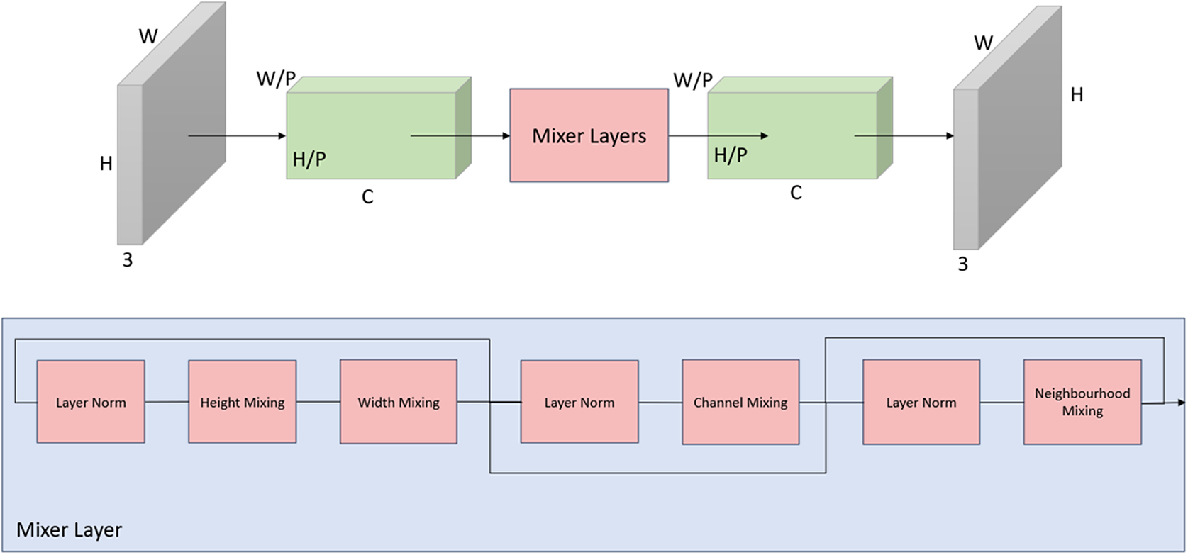
Figure 2. A schematic representation of the proposed modified image-to-image mixer model adapted from (Mansour et al., Reference Mansour, Lin and Heckel2023). Details of the mixing layers are shown underneath.

2.6. Compute resource

The training and hyperparameter tuning processes were conducted on a Linux machine, leveraging the computational power of a single A100 GPU, accompanied by 16 CPU cores and 64GB RAM. The model underwent training for a total of 20 epochs, taking approximately 8 hours.

3.1. Qualitative comparison to CFD

From a qualitative perspective, we compared the model-generated flow patterns to those produced by CFD simulations. This evaluation aimed to assess the model’s capability to capture the expected physical behavior of the wind, particularly in areas characterised by high wind velocity amplification, often associated with increased discomfort and risk to pedestrians. This qualitative assessment involved a visual inspection of model predictions alongside the corresponding ground truth for each velocity component and magnitude. An illustrative example of this comparison is presented in Figure 3. Notably, the model exhibits proficiency in replicating key features around the geometry, including small areas of stagnation at the leading edge of the geometry and the wake region on the leeward side. As the wind circulates around the outer perimeter of the geometry, the model accurately captures regions of high velocity, particularly in gaps between buildings. Additionally, the model successfully reproduces amplified flows penetrating from the outer edge through canyons formed between buildings. In areas where courtyards exist, characterised by open spaces surrounded by buildings, the model appropriately reflects the increase in wind flow. Toward the centre of the geometry, the model demonstrates its ability to predict heightened flow velocities between buildings, even far from the free stream, after undergoing complex interactions.

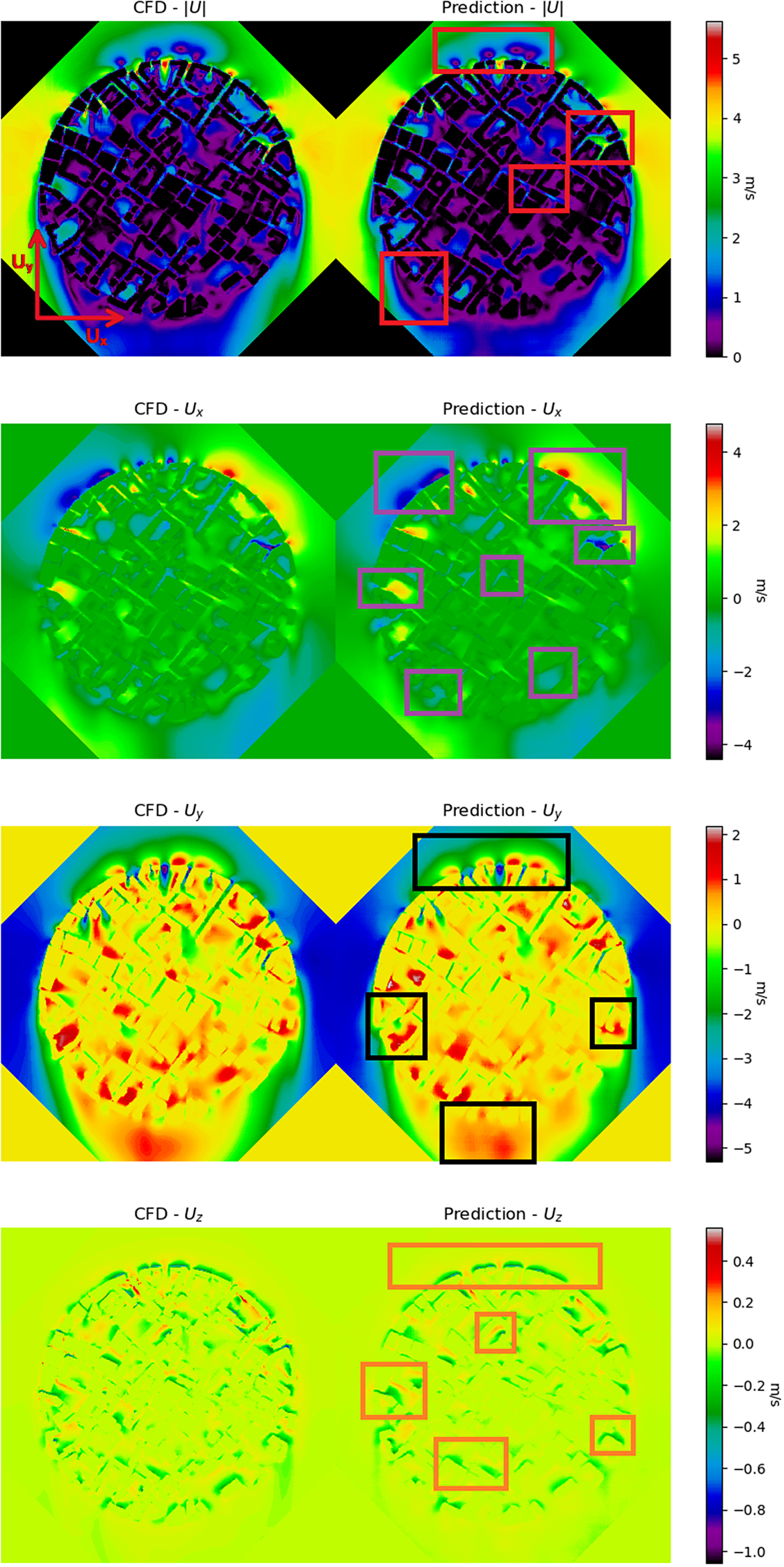
Figure 3. A qualitative comparison between the predicted flow field generated by the deep learning model and the corresponding CFD simulation. Highlighted areas pinpoint instances where the model successfully replicates essential features of the wind flow, providing valuable insights into its performance.

Upon examining individual velocity components, the model effectively captures the majority of significant flow features for both the $ {U}_x $ and $ {U}_y $ directions. Particularly noteworthy is the model’s accurate representation of the reversal of flow direction in the $ {U}_y $ component, observed in the wake region and on the windward side of the geometry. An analysis of the $ {U}_z $ component reveals the model’s success in reproducing downwash on the windward side of the buildings throughout the entire geometry. The agreement between the model and the ground truth is reasonably high for the $ z $ -components, which aligns with expectations due to the naturally lower velocities associated with this component.

3.2. Quantitative comparison to CFD

To quantify the model’s performance, we initially plot the error $ \parallel {y}_i\parallel -\parallel f\left({x}_i,\theta \right)\parallel $ normalised by the reference velocity at a height of 2 m shown in Figure 4. In general, the model demonstrates commendable performance across the domain, with low errors typically falling within the range of $ \pm 0.625 $ m/s. However, it becomes evident that while the majority of flow features are effectively captured, the precise shapes of these features and the predicted associated wind velocities can exhibit errors in the region of 2 m/s with rare occurrences exceeding 3.5 m/s. The level of under/over-prediction by the model is not consistent throughout the domain, displaying no clear pattern.

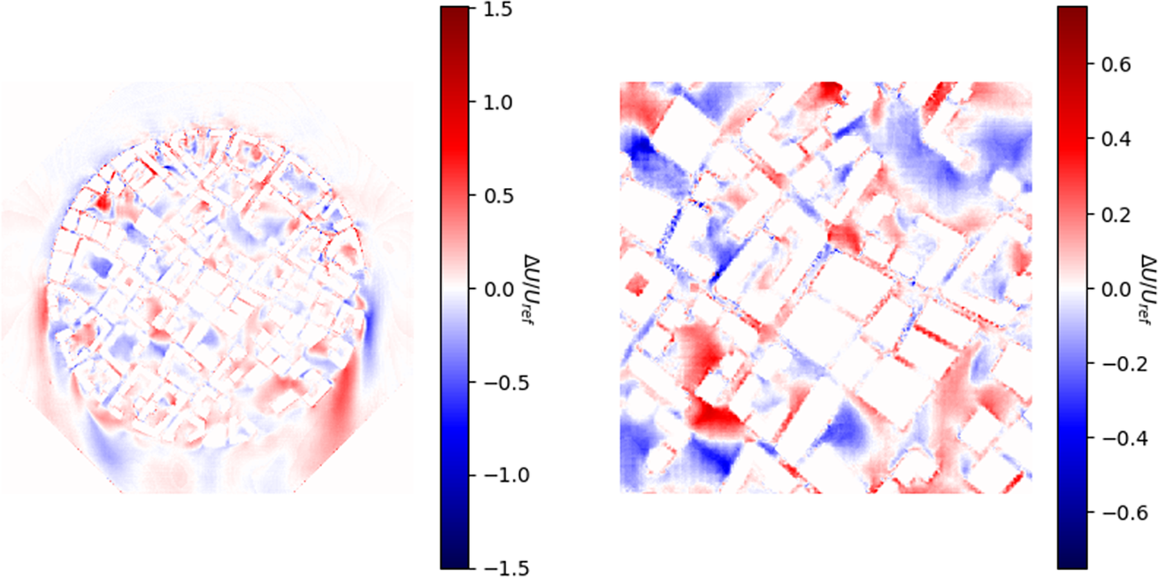
Figure 4. Error plots depicting the difference between the predicted magnitude generated by the deep learning model and the simulated magnitude from CFD for the entire image and the centre section. The magnitude difference is normalised by the reference velocity at a 2 m height.

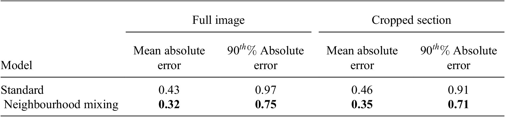
The findings from the error plots are further supported by descriptive statistics provided in Table 1.

Table 1. Performance comparison between the standard MLP mixer and the modified version measured on the test set. Mean absolute errors and the 90th percentile absolute errors for the entire image and the centre section, excluding building or masked corner pixels, provide insights into the accuracy and robustness of each model in predicting pedestrian-level wind conditions. Lower errors indicate superior performance.

3.3. Effect of neighbourhood mixing

Comparison between a model equipped with a neighbourhood mixing layer to the standard unmodified architecture reveals significant enhancements across all error metrics and in the representation of flow patterns. The quality of the comparison is particularly marked by a reduction in pixel-wise errors and effective mitigation of discontinuities in the generated flow fields. Moreover, the standard mixer exhibits a tendency to introduce artifacts into the generated image, implying valuable information can be captured in the immediate local area. Omitting this information leads to confusion and the presentation of behaviors that contradict physical laws such as discontinuities in the flow field. These improvements signify the efficacy of the introduced architectural modification in refining the model’s ability to generate more accurate and coherent representations of wind behaviour. Consequently, this enhancement contributes to an overall improvement in the model’s performance and predictive capabilities, which is clearly depicted in Figure 5.

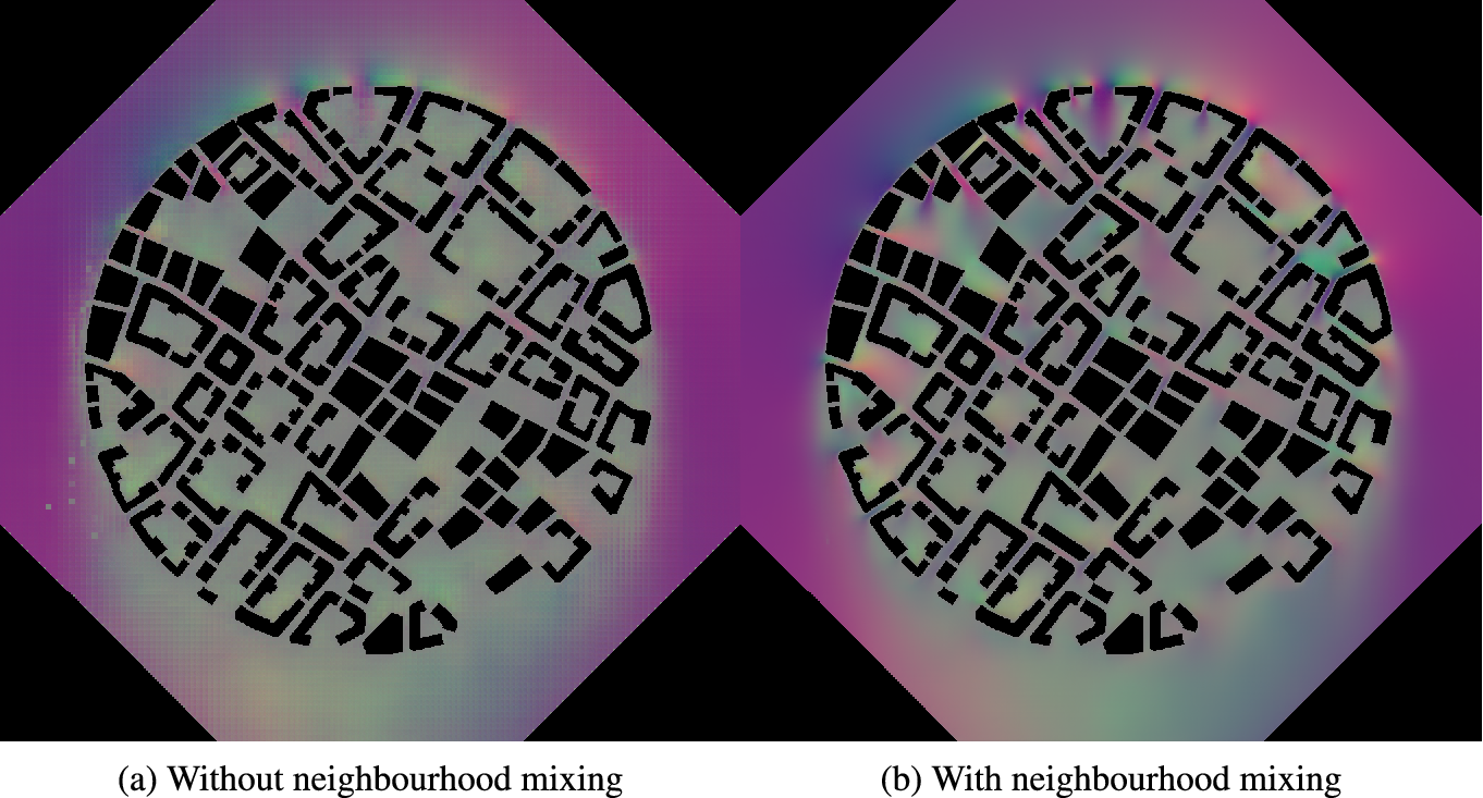
Figure 5. A side-by-side comparison of the predicted flow fields produced by the standard mixer model (a) and the proposed modified version (b).

3.4. Effect of training set size

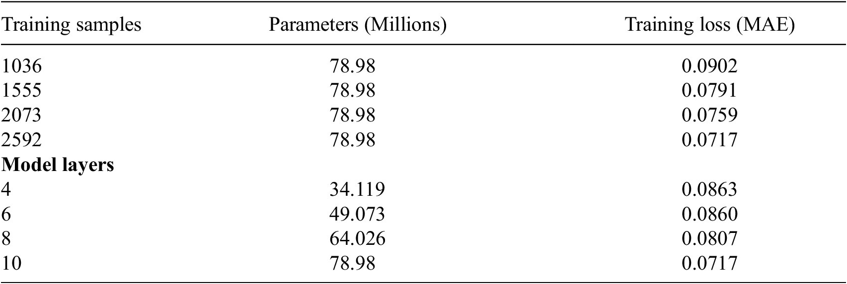
Deep learning models are inherently shaped by the data they are trained on, making the volume and quality of the training dataset pivotal factors in determining model performance. In our study, we explore the impact of training set size by comparing models trained on varying proportions of the total dataset: 100%, 80%, 60%, and 40%. The mean absolute error (MAE) for each trained model is documented in Table 2. Notably, the largest decrease in loss is observed between the models trained on 40% and 60% of the dataset, indicating the importance of sufficient data for model effectiveness. Furthermore, as the proportion of training samples increases, there is a consistent linear decrease in loss, underscoring the direct correlation between data volume and model performance.

Table 2. Top: Influence of training set size on model performance. Bottom: Influence of model size on performance

Despite these improvements, our analysis suggests that there remains potential for further enhancement, particularly through the expansion of the training dataset. Increasing the size of the training set could offer additional opportunities for refining model accuracy and generalisation, thereby optimising performance in PLW assessment tasks.

3.5. Effect of model size

We conducted training iterations of the model using different numbers of layers: 4, 6, 8, and 10. Interestingly, models with 4 and 6 layers exhibited comparable performance, with minimal disparity in MAE loss. However, as additional layers were added, the loss demonstrated a further decrease, suggesting the potential for continued improvement with larger models.

It is noteworthy, however, that increasing the number of layers introduces a risk of overfitting, particularly when working with a relatively small dataset. As the model parameters expand, so does the susceptibility to overfitting, where the model may excel in learning from the training data but struggle to generalise effectively to unseen data.

3.6. Inference time

CFD studies are known to be time-intensive. The data generated for model training and testing took 80–100 minutes to resolve a single training example. In contrast, our developed deep learning model achieves remarkable efficiency, with an average inference time of just 0.008 seconds per forward pass. This significant speed enhancement is particularly advantageous considering the multitude of wind directions that must be simulated for each design iteration in a PLW assessment. Consequently, our model holds considerable promise as a rapid and effective tool for preliminary design assessments, offering substantial time savings over traditional CFD approaches.