2.1 Experimental market

The lab environment is based on an asset pricing model with heterogeneous beliefs following Brock and Hommes (Reference Brock and Hommes1998); for a textbook treatment see Campbell et al. (Reference Campbell, Lo and MacKinlay1997). Consider an asset market with heterogeneous beliefs where agents need to allocate their wealth between a risk-free bond (that pays gross return of $R=1+r$ ) and a risky asset that pays an uncertain dividend with an average dividend of $\overline{y}$ . Based on this allocation decision, the wealth of agent i in period $t+1$ is given by

(1) $\begin{array}{c}{W}_{i,t+1}=R{W}_{i,t}+z_{i,t}(p_{t+1}+y_{t+1}-R{p}_t),\end{array}$

where $z_{i,t}$ is the position of the risky asset by agent i in period t (positive or negative) and $p_t$ and $p_{t+1}$ are the prices of the risky asset in periods t and $t+1$ respectively. We assume that agents maximize a simple myopic mean-variance utility function, that is, they solve the following problem:

(2) $\begin{array}{c}\underset{z_{i,t}}{max}\left(E_{i,t},W_{i,t+1},-,\frac{a}{2},V_{i,t},\left(W_{i,t+1}\right)\right)\equiv \underset{z_{i,t}}{max}\left(z_{i,t},E_{i,t},{\rho }_{t+1},-,\frac{a}{2},z_{i,t}^2,V_{i,t},\left({\rho }_{t+1}\right)\right),\end{array}$

where $E_{i,t}$ and $V_{i,t}$ are the individual expectations about wealth and variance. Note that these might not be perfectly rational. Furthermore, a is a parameter for risk aversion, and ${\rho }_{t+1}$ is the excess return defined as ${\rho }_{t+1}\equiv p_{t+1}+y_{t+1}-R{p}_t$ . For simplicity we assume that the expected variance of excess return is constant and homogeneous across agents, i.e. $V_{i,t}\left({\rho }_{t+1}\right)={\sigma }^2$ . Given these assumptions the optimal demand of agent i is given by

(3) $\begin{array}{c}{z}_{i,t}^{\ast }=\frac{E_{i,t}\left({\rho }_{t+1}\right)}{a{V}_{i,t}\left({\rho }_{t+1}\right)}=\frac{p_{i,t+1}^e+\overline{y}-R{p}_t}{a{\sigma }^2},\end{array}$

where $p_{i,t+1}^e=E_{i,t}\left(p_{t+1}\right)$ is the individual forecast by agent i of the price in period $t+1$ and $\overline{y}=E_t\left[y_t\right]$ is the forecast of the exogenous dividend process $y_t$ , assumed to be correct for all agents. The market price for the risky asset is set by market clearing, that is demand equals supply:

(4) $\begin{array}{c}\sum _{i=1}^N{z}_{i,t}^{\ast }=Z_t^S,\end{array}$

where $Z_t^S$ is the exogenous supply. For simplicity, we assume that this exogenous supply is 0. Furthermore we assume a small fraction of noise traders. Their position is incorporated in the equilibrium pricing equation as a small IID noise term, ${\epsilon }_t\sim N(0,0.5)$ . This results in an equilibrium pricing equation

$\begin{array}{c}{p}_t=\frac{1}{(1+r)N}\left(\sum _{i=1}^N,\left(E_{i,t},\left(p_{t+1}\right),+,\overline{y}\right)\right)+{\epsilon }_t=\frac{1}{(1+r)}\left({\overline{p}}_{t+1}^e,+,\overline{y}\right)+{\epsilon }_t,\end{array}$

or equivalently

(5) $\begin{array}{c}{p}_t=p^f+\frac{1}{1+r}({\overline{p}}_{t+1}^e-p^f)+{\epsilon }_t,\end{array}$

where ${\overline{p}}_{t+1}^e$ is the average forecast for period $t+1$ across all individuals.

Note that the realized price $p_t$ in period t depends on the average prediction ${\overline{p}}_{t+1}^e$ for period $t+1$ and agents use information up to period $t-1$ when predicting the price of $t+1$ , so all forecasts are two periods ahead. Also note that the rational expectation equilibrium is that agents expect the price to be equal to the fundamental price, $p^f=\overline{y}/r$ . In that case, the law of motion for the price becomes $p_t=p^f+{\epsilon }_t$ , so that expectations are self-fulfilling. In the experiment, we use the following parameters: $\overline{y}=3.3$ and $R=1.05$ . This implies that the fundamental price is 66.

Notice also that the price equation (5) has rational bubble solutions, where the deviation from the fundamental price $x_t=p_t-p^f$ grows at the risk-free rate r. In theory, these rational bubbles are often excluded by a transversality condition.

2.2 Implementation

In the experiment subjects are playing the role of a financial advisor of a pension fund. They are informed that they have to forecast the price of a risky asset, and that based on their forecast, the pension funds will have a certain demand of the asset. They are not explicitly told the law of motion (5), but they know that there is positive feedback in the market (i.e., the higher their forecast is, the higher the realized price will be ceteris paribus). The market lasts 50 periods.

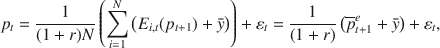
Subjects are only paid according to their forecasting performance. Their payoff is determined by the following formula:Footnote ⁸

(6) $\begin{array}{c}\text{Payoff}{}_{i,t+1}=max\left(0,,,\left(1300,-,\frac{1300}{49},{\left(p_{i,t+1}^e,-,p_{t+1}\right)}^2\right)\right),\end{array}$

where $p_{i,t+1}^e$ denotes the forecast of the price at period $t+1$ formulated by subject i in period t without knowing $p_t$ , and $p_{t+1}$ is the realised asset price at period $t+1$ . Subjects were informed about this payoff function, and they were also provided a payoff table showing earnings corresponding to given forecast errors. Subjects accumulated their payoffs during the experiment, which was converted to euros at the end. They received 0.5 euro for each 1300 points they earned.

During the experiment subjects could see past prices, their own actions and whether they received news in a given period, but not others’ decisions. As in previous experiments (see e.g. Hommes et al. Reference Hommes, Sonnemans, Tuinstra and van de Velden2008), we did not explicitly tell subjects the fundamental price, but they are informed about the average dividend, $\overline{y}$ and the risk free interest rate r, thus they would have been able to calculate the fundamental price as $p^f=\overline{y}/r$ .

In order to control huge deviations from the fundamental price, we imposed an upper limit of 1000 on the forecasts. Subjects became only aware of this once they tried to submit a forecast higher than 1000.Footnote ⁹ They would receive an error message in that case and had to reenter a forecast $\le$ 1000. As a new experimental design feature, we introduced news announcements which stated either “Experts say the stock market is overvalued” or “Experts say the stock market is undervalued”. When the price was more than 3 times the fundamental price, or when it was lower than $\frac{1}{3}$ of the fundamental price, the news announcement appeared on screen with 25% probability for each subject (independently drawn). Subjects were told that “When there is news, on average only 1 out of 4 subjects will receive news.” This procedure was employed in all periods, so when the price was far from fundamental price for several periods in a row, it could be that a subject did not get the news in one of the first periods but only later (or never), and it could be that a subject did receive news in a period but not in the subsequent one although the price was even farther away from the fundamental price. This way the direct effect of the news on individual behaviour can be measured, as in each round when the news was depicted, there were some subjects receiving it, and others not.Footnote ¹⁰ For an example of the news, see Supplementary material online Appendix. Finally, in order to prevent huge variation in initial predictions, subjects were told that the price in the first period is very likely to be between 0 and 100.

2.3 Treatments and experimental procedure

Large groups around 100 do not fit into a single lab. Therefore, the experiment was conducted by connecting the experimental CREED-lab in Amsterdam and the LINEEX-lab in Valencia via internet. All participants knew this and they could choose between English and Spanish at the beginning of the session. The experiment was programmed in php. In the first 6 sessions all subjects formed one large market, whereas in the $7^{\mathrm{th}}$ session subjects were grouped in markets of 6. This results in total in 6 large markets and 13 small markets.Footnote ¹¹ In total 676 (370 in Valencia and 306 in Amsterdam) subjects participated, mainly students with various backgrounds.

In order to keep the length of the experiment within a reasonable time span, a time limit on the decisions was imposed. Subjects had 2 min to make a decision in the first 10 periods, and 1 minute in later periods. If subjects did not submit a decision on time, they would not earn anything that period, and the average forecast was determined based only on the other forecasts.Footnote ¹² Before the experiment, subjects had the opportunity to read the instructions at their own pace from the computer screen, which took on average 40 min until everyone completed. The experimental market took on average 1 hour per session. The English instructions are presented in Supplementary material online Appendix (the Spanish instructions are available upon request). Subjects earned on average 8.3 euros from the forecasting task (with a minimum of 0 and a maximum of 21.84 euros out of 25 euros) plus a show-up fee, plus additional earnings from an unrelated, surprise one-shot volunteer’s dilemma after the experimental asset market (Kopányi-Peuker Reference Kopányi-Peuker2019).Footnote ¹³

3.1 Market behaviour

Figure 1 shows the market price for each market in the 13 small groups (left panel) and the 6 large groups (right panel).Footnote ¹⁴ The time evolution of the market price is very heterogeneous across groups for both the Small and the Large treatments. We distinguish three different qualitative market behaviours:

1. (i) markets which are stable or exhibit small oscillations around the fundamental price;

2. (ii) markets with moderately large bubbles, with a peak at about 3-4 times the fundamental price, so that some subjects receive news, but the bubble does not reach the exogenous upper bound; and

3. (iii) markets with very large bubbles, with a peak of more than 10 times fundamental price, and a crash because some subjects reached the highest possible forecast of 1000.

Table 1 contains descriptive statistics about each market by presenting the median and mean market price, the standard deviation and the relative (absolute) deviation from the fundamental price. The markets are ranked according to their median price. For the small group size there are five stable markets (the first five groups in Table 1), six markets with moderately large bubbles (groups 6 to 13 in Table 1) and two markets with very large bubbles (groups 10 and 11). For the large group size there are three stable markets (groups 92, 103 and 100-1), one with a moderately large bubble (group 99) and two with very large bubbles (groups 100-2 and 104). Markets which have a relative low average/mean price also have a relative low standard deviation and are thus more stable. Other markets are heavily overpriced, and they also have rather high standard deviation due to the observed bubbles and crashes.

Fig. 1 Realized prices in each market for the Small (left panel) and the Large (right panel) treatments

Table 1 Descriptive statistics of the markets

group ID	Median	Mean	SD	RAD	RD	IE	DE (%)	CE (%)
Group 5	42.77	42.86	11.31	35.06	$-35.06$	284.51	238.87 (84%)	45.64 (16%)
Group 2	54.89	55.11	19.29	27.79	$-16.49$	483.81	222.93 (46%)	260.89 (54%)
Group 4	57.04	59.71	20.48	28.14	$-9.52$	337.00	99.71 (30%)	237.29 (70%)
Group 8	60.47	60.80	4.72	8.72	$-7.87$	21.99	18.98 (86%)	3.01 (14%)
Group 7	74.84	78.82	24.43	27.21	19.43	1771.99	1458.85 (82%)	313.14 (18%)
Group 6	84.06	90.22	57.85	66.23	36.70	1187.87	568.26 (48%)	619.62 (52%)
Group 12	93.43	131.60	109.91	133.14	99.39	4645.08	1707.59 (37%)	2937.49 (63%)
Group 1	102.80	113.88	51.93	78.31	72.55	6558.04	5264.37 (80%)	1293.67 (20%)
Group 9	126.69	137.01	75.66	118.99	107.59	7535.47	4948.32 (66%)	2587.15 (34%)
Group 3	129.98	177.02	135.13	196.50	168.21	4533.43	3571.60 (79%)	961.83 (21%)
Group 13	173.62	248.54	211.17	297.85	276.57	2806.46	366.89 (13%)	2439.57 (87%)
Group 11	208.93	352.15	308.03	446.66	433.56	27174.41	6084.24 (22%)	21090.17 (78%)
Group 10	392.88	446.54	323.79	588.97	576.58	21681.09	6239.74 (29%)	15441.35 (71%)
Group 92	63.28	62.54	5.18	7.59	$-5.24$	1318.73	1302.24 (99%)	16.49 (1%)
Group 103	69.11	68.59	4.48	6.54	3.92	438.90	428.74 (98%)	10.16 (2%)
Group 100-1	69.57	64.29	26.15	33.45	-2.60	395.72	111.22 (28%)	284.50 (72%)
Group 99	84.75	104.12	72.22	87.63	57.76	3830.15	2113.17 (55%)	1716.98 (45%)
Group 100-2	106.45	271.20	284.78	333.29	310.90	24772.46	8258.59 (33%)	16513.94 (67%)
Group 104	133.27	265.55	275.71	325.37	302.35	20786.80	8482.93 (41%)	12304.50 (59%)

Groups 1–13 are the small groups with group size 6, and groups 92 to 104 are the large markets. For these markets, the number in the group ID indicates the number of subjects forming that market. Markets are sorted on Median market price. RAD (Relative Absolute Deviation) and RD (Relative Deviation) are in percentages, and are calculated by the average (absolute) deviation from the fundamental price divided by the fundamental price. Average individual forecast errors (IE) are calculated by taking the average over individuals and periods of the individual quadratic forecast errors. Dispersion error (DE) is calculated by taking the average of the quadratic differences between individual forecasts and the average forecast for a given period. Finally, common error (CE) is calculated by taking the average of the quadratic difference between the average forecast and the realized price. Note that $IE=DE+CE$

The overall average market price over the 50 periods per treatment is 139.38 for the Large groups and 153.41 for the Small groups (this difference is not statistically significant, $p=0.93$ ).Footnote ¹⁵ Furthermore, in the Small treatment the average price is significantly higher than the fundamental price of 66 ( $p=0.02$ according to the Wilcoxon signrank test), whereas the average price is not significantly higher than 66 for the Large groups ( $p=0.17$ ; n = 6).Footnote ¹⁶ All markets’ standard deviations are significantly higher than the standard deviation predicted by the rational expectation model, that is, the $SD=0.5$ of the noise term ${\epsilon }_t$ in (5), so all markets exhibit significant excess volatility.

Table 1 also reports the Relative Absolute Deviation (RAD) and the Relative Deviation (RD) from the fundamental price.Footnote ¹⁷ Most markets are overpriced, but there is no market in which the price never goes under the fundamental price. There is one market in which the price is constantly under the fundamental price: group 5 in the Small treatment (group 8 shows almost the same pattern). The most stable groups 92, 103 and 8 (in terms of SD) stay quite close to the fundamental price (with relatively low RAD and RD), but the stable group 100-1 oscillates around $p^f$ (with relatively high RAD compared to RD). In markets with bubbles both RAD and RD are relatively high. To sum up, based on the qualitative market price behaviour and these summary statistics, no striking differences between the aggregate behaviour in small and large groups can be observed.Footnote ¹⁸

3.2 Coordination of expectations

Do subjects manage to coordinate their expectations in a market or does heterogeneity prevail? Figure 2 shows time series plots of the coefficient of variation of individual forecasts, that is, the standard deviation divided by the mean, for the small and the large markets. A low (high) value of the coefficient of variation corresponds to a high (low) degree of coordination of forecasts. Heterogeneity strongly fluctuates over time with many high peaks. In the small groups, the time variation seems somewhat noisier, with many sudden high peaks perhaps due to individual experimentation. In the large groups heterogeneity seems to vary more smoothly and gradually, although there are still some sudden high peaks. In any case, we do not observe stronger coordination towards the end of the experiment, but for most markets heterogeneity continues to fluctuate over time.

Fig. 2 Coefficient of variation of individual predictions (standard deviation divided by the mean) in each market for the Small (left panel) and the Large (right panel) treatments. A low (high) value means that individual forecasts are strongly (weakly) coordinated

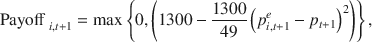
To study the time-varying heterogeneity in more detail, Figs. 3, 4 and 5 plot typical examples of the three different types of market behavior for both small and large markets. These figures show the market price together with the coefficient of variation of individual predictions. Figure 3 illustrates a typical example of a stable market; Fig. 4 of moderately large bubbles, and Fig. 5 of very large bubbles.Footnote ¹⁹ The blue solid lines correspond to the market price and are depicted on the left vertical axis; the red dashed lines correspond to the coefficient of variation of individual forecasts and are measured on the right vertical axis.

Fig. 3 Market price (left scale) and coefficient of variation of individual forecasts (right scale) for examples of stable markets in a small (left) and a large (right) group

Fig. 4 Market price (left scale) and coefficient of variation of individual forecasts (right scale) for examples of moderately large bubbles in a small (left) and a large (right) market

Fig. 5 Market price (left scale) and coefficient of variation of individual forecasts (right scale) for examples of very large bubbles in a small (left) and a large (right) market

In the stable markets (Fig. 3) after an initial phase of high heterogeneity and some initial fluctuations, the heterogeneity drops almost to zero after about 15 periods. Subjects thus learn to coordinate their expectations within 15 periods and in both the small and large markets the price exhibits small fluctuations close to the fundamental value. Compared to the other markets, coordination of expectations is the strongest in the stable markets.

In the markets with moderately large bubbles (Fig. 4) heterogeneity is initially high, but quickly drops to lower levels. The market price is above fundamental value, however, and starts to increase further. In the small market (left panel in Fig. 4) the price starts following a strong upward trend and heterogeneity gradually increases. The market price increases and peaks around 400 in period 15, after which the market crashes and heterogeneity increases rapidly and sharply. The pattern in the large market is somewhat different (right panel in Fig. 4), where first a small bubble with a peak around 100 at period 10 occurs, followed by a decline to very low prices around period 20, followed by a larger bubble with a peak around 200 in period 30. After the first small bubble and crash, heterogeneity increases substantially and remains high during the second bubble and crash.

Figure 5 illustrates the time variation of heterogeneity in markets with very large bubbles. Initially heterogeneity is high, but quickly drops to low levels within 5 periods, after which heterogeneity gradually increases along the large bubbles. After the market crash heterogeneity peaks and remains high illustrating a state of confusion among subjects. This pattern of time variation of heterogeneity and coordination is particularly clear and smooth in the large market (right panel in Fig. 5), but it also occurs in the small market, although the pattern is noisier there due to more individual uncertainty in small groups. We conclude from this pattern that strong coordination of expectations amplifies the large bubbles and that after a market crash heterogeneity (confusion) remains high. In Supplementary material online Appendix we fit the behavioural heuristics switching model (HSM) of Anufriev and Hommes (Reference Anufriev and Hommes2012) to the experimental data and show that coordination on a trend-following heuristic amplifies bubbles in small and in large markets.

To further quantify the coordination between subjects, we have calculated the average quadratic individual error (IE), the dispersion error (DE) and the common error (CE) for each market. IE is calculated by taking all individual quadratic forecast errors for each period in which a forecast was submitted, and then taking the average of all these forecasts over individuals and periods for each market ( $\text{IE}=\frac{1}{K}{\sum }_{t,i}{(p_{i,t}^e-p_t)}^2$ , where K is the number of individual forecasts in a group in all 50 periods). This error measures how well subjects predict the market price. The dispersion error is calculated by taking the average of the quadratic difference of the individual forecasts and the average forecast of the given period over all individuals and periods for each market ( $\text{DE}=\frac{1}{K}{\sum }_{t,i}{(p_{i,t}^e-{\overline{p}}_t^e)}^2$ , where K is the same as before). DE measures how well subjects coordinate with each other. Finally, the common error (CE) is calculated by taking the average quadratic error of the mean forecast compared to the realized price ( $\text{CE}=\frac{1}{50}{\sum }_t{({\overline{p}}_t^e-p_t)}^2$ ). The common error measures the quality of the average expectations. Table 1 presents IE, DE and CE for each market. By definition $IE=DE+CE$ . Because of this it is easy to see that DE and CE cannot easily be interpreted in absolute terms, but only relative to IE. This is because in a more stable market IE tends to be much smaller than in less stable markets. There is a huge variation across markets whether the common or the dispersion errors are relatively large within the individual errors. However, a relatively small common error is more common in the more stable groups. The correlation between the standard deviation of the marketprice and the percentage of CE compared to IE is 0.71 ( $p=0.00$ according to the Spearman rank correlation test). This means that in these more stable markets individual errors tend to cancel out (although of course not perfectly). This happens both in small and large groups. The percentage of CE compared to IE is not significantly different in small and large groups ( $p=0.66$ according to the ranksum test). This finding is in line with Muth (Reference Muth1961), who stated that even though individuals make prediction errors, on average they make rational decisions when individual errors are likely to cancel out. In markets with large bubbles CE is much larger than DE. Thus, in these markets aggregate expectations are not rational in the sense of Muth (Reference Muth1961).

3.3 News announcements

Does news about the over- or undervaluation affect individual expectations and aggregate behaviour? In particular, can news break the coordination on a bubble? News appeared with probability 25% when the last price was sufficiently far away from the fundamental price, either below 1/3 or above 3 times fundamental value. For practical reasons, our analysis focuses only on overvaluation.Footnote ²⁰

News of overvaluation was observed in 8 small groups (from Group 6 onwards in Table 1) and in 3 large groups (from Group 99 onwards in Table 1). Table 2 shows the average relative increase in individual predictions after the first news element is seen in a group, for each bubble separately for those who have seen the news, and those who have not seen the news.Footnote ²¹ The data is pooled for small and large markets. In all bubbles the participants who received the news increase their prediction less than those who did not receive the news. We first test the statistical significance in a quite conservative way in which the level of observation is the individual group, and the data is the average relative change in prediction of the participants who did or did not receive the news. This means that we have only few data-points and thus a low statistical power. Nevertheless, a Wilcoxon test shows (two-sided) p-values of $p<0.01$ for bubble 1 and $p=0.05$ for bubble 2 and 3. Note that in this analysis small and large groups are pooled. To study a treatment effect and possible interaction effects we run regressions, as shown in Table 3. We find significant effect for the news, and no effects for the treatment small/large. These results are the same for all three bubbles combined, or the first two separate bubbles. For bubble 3, with relatively few observations, the effect of the news is not statistically significant.

Another striking feature of Tables 2 and 3 is that the average increase in predictions substantially grows from the first to the second bubble. It looks as if the first bubble is generally slower than later bubbles when subjects already gained experience with bubbles, crashes, and the news element. However, these differences are not statistically significant at conventional levels.

Table 2 Average relative increase in prediction (change of prediction divided by the last prediction) after the first news-element is seen in the group for the different bubbles over time—all data

	1st bubble	2nd bubble	3rd bubble
No news	26.8% (46.3)	92.3% (130.9)	100.6% (130.4)
News	7.7% (24.6)	60.4% (87.8)	57.6% (147.8)
# of markets	11	8	7

Table contains averages over individuals for both small and large markets

Table 3 Regressions per bubble on the relative increase in prediction

Dependent variable: Relative increase in prediction
	First 3 bubbles	1st bubble	2nd bubble	3rd bubble
News	−0.25*** (0.08)	−0.16*** (0.03)	−0.30** (0.12)	−0.30 (0.18)
Size	0.07 (0.35)	0.41 (0.33)	−0.35 (0.39)	0.20 (0.84)
News*size	−0.28 (0.16)	−0.27 (0.25)	−0.06 (0.23)	−0.65 (0.42)
Constant	0.69** (0.28)	0.22*** (0.04)	0.95** (0.33)	0.99 (0.56)
# of observations	893	341	325	227
# of markets	11	11	8	7

***: significant at 1%-level, **: significant at 5%-level. Dependent variable is the relative change in prediction (change of prediction divided by the last prediction). News = 1 if the participant received news, Size = 1 if the groups size is small. Only rounds when the first news in a bubble was depicted are considered. Standard errors are in brackets and clustered on the market level. Bubbles number 4 and 5 are dropped, due to limited number of markets

News of overvaluation thus has a significant effect on individual expectations: it leads to significantly lower increase in forecasts along the first bubble. Does this effect of news on individual behaviour translate into an aggregate effect and stabilize the bubble? We compare our markets with earlier LtF markets that did not have a news- element in their design. We focus only on groups that have received news in our experiment (8 small and 3 large groups) and the markets in three earlier LtF experiments in which participants would have received news in our setup. All these markets have bubbles, and we define a bubble to be extreme if the market price almost hits the upper bound. In the present experiment 4/11 bubbles are extreme (2 small and 2 large market). In Hommes et al. (Reference Hommes, Sonnemans, Tuinstra and van de Velden2008) 5/6 bubbles are extreme; in Bao et al. (Reference Bao, Hennequin, Hommes and Massaro2020) 6/7 bubbles are extreme; and in Kopányi-Peuker and Weber (Reference Kopányi-Peuker and Weber2019) 5/8 bubbles are extreme. Combining these no-news markets we get a 16/21 proportion of extreme markets, which is statistically significant more than the 4/11 proportion in the present experiment (one-sided proportion test $p=0.014$ ). This is not the most elegant way to compare the effect of news on market stability (future research could direct compare markets with and without news), but this data suggests strongly that news did have an effect, not only at an individual level but also at the aggregate level of markets.