2. Problem formulation

Consider flow in a slot driven by movement of the upper plate with a prescribed velocity $U_{top}$ while the lower plate is stationary. The slot extends to $\pm \mathrm{\infty }$ in the X- and Z-directions with plates placed at a distance $2h$ apart, as shown in figure 1. The lower plate is exposed to vibrations in the form of a sinusoidal travelling wave, resulting in the time-dependent slot geometry of the form

(2.1) \begin{equation}Y_{L }(t,X)=-1+\tfrac{1}{2}\cos[\alpha \left(X-ct\right)],\end{equation}

where subscript $L$ refers to the lower plate, and $h$ was used as the length scale.

Figure 1. Schematic diagram of the flow system.

The velocity vector $\boldsymbol{{V}}=(u,v,w)$ is scaled with the viscous velocity scale $U_{v}=v/h$ , the pressure $p$ is scaled with $\rho U_{v}^{2}$ (where $\rho$ denotes the fluid density), and the time $t$ is scaled with $h/U_{v}$ . The relevant boundary conditions are

(2.2a–f) \begin{equation}\text{for }Y=1,\quad u=Re,\ v=0,\ w=0,\qquad \text{for }Y=Y_{L}(t,X),\quad u=0,\ v=\frac{\partial Y_{L}}{\partial t},\ w=0,\end{equation}

where

(2.3) \begin{equation}Re\equiv U_{top}h/\nu\end{equation}

is the Reynolds number. Since the flow is driven solely by the movement of the upper plate, the pressure gradient constraint in the form

(2.4) \begin{equation}\left.\frac{\partial p}{\partial X}\right| _{m}=0,\end{equation}

where subscript m denotes the mean value, must be imposed.

It is simpler to carry out detailed calculations using the frame of reference moving with the wave, which leads to Galileo’s transformation of the form

(2.5a–c) \begin{equation}x=X-ct,\quad y=Y,\quad z=Z.\end{equation}

The complete problem formulation can now be written as

(2.6a) \begin{equation}\frac{\partial u}{\partial t}+\left(u-c\right)\frac{\partial u}{\partial x}+v\frac{\partial u}{\partial y}+w\frac{\partial u}{\partial z}=-\frac{\partial p}{\partial x}+\frac{\partial ^{2}u}{\partial x^{2}}+\frac{\partial ^{2}u}{\partial y^{2}}+\frac{\partial ^{2}u}{\partial z^{2}},\end{equation}

(2.6b) \begin{equation}\frac{\partial v}{\partial t}+\left(u-c\right)\frac{\partial v}{\partial x}+v\frac{\partial v}{\partial y}+w\frac{\partial v}{\partial z}=-\frac{\partial p}{\partial y}+\frac{\partial ^{2}v}{\partial x^{2}}+\frac{\partial ^{2}v}{\partial y^{2}}+\frac{\partial ^{2}v}{\partial z^{2}},\end{equation}

(2.6c) \begin{equation}\frac{\partial w}{\partial t}+\left(u-c\right)\frac{\partial w}{\partial x}+v\frac{\partial w}{\partial y}+w\frac{\partial w}{\partial z}=-\frac{\partial p}{\partial z}+\frac{\partial ^{2}w}{\partial x^{2}}+\frac{\partial ^{2}w}{\partial y^{2}}+\frac{\partial ^{2}w}{\partial z^{2}},\end{equation}

(2.6d) \begin{equation}\frac{\partial u}{\partial x}+\frac{\partial v}{\partial y}+\frac{\partial w}{\partial z}=0,\end{equation}

(2.6e–g) \begin{equation}\text{for }y=1,\quad u=Re,\ v=0,\ w=0,\end{equation}

(2.6h–j) \begin{equation}\text{for }y=y_{L}(x)=-1+\frac{1}{2}\cos[\alpha (X-ct)],\quad u=0,\ v=-c\,\frac{{\rm d}y_{L}(x)}{{\rm d}x},\ w=0,\end{equation}

(2.6k) \begin{equation}\left.\frac{\partial p}{\partial x}\right| _{mean}=0.\end{equation}

The next section begins with a detailed analysis of the two-dimensional stationary state in the moving reference frame.

3. Determination of the primary state

The primary state has the form of a two-dimensional stationary flow in the moving frame of reference, i.e. $w=0$ , ${\partial }/{\partial z}=0$ , ${\partial }/{\partial t}=0$ . This flow is expected to bifurcate to a secondary state consisting of streamwise vortices. This analysis aims to determine critical conditions leading to such a bifurcation. We begin with a discussion of the properties of the stationary state before proceeding to stability analysis.

3.1. Problem formulation and numerical solution

The translation of the upper plate in the absence of any vibrations creates a simple Couette flow. The velocity field $\boldsymbol{v}_{\mathbf{0}}$ , pressure $p_{0}$ , pulling force applied to the upper plate (per unit length and width) $F_{0}$ , shear acting on the upper plate $\tau _{0}$ , and flow rate $Q_{0}$ are given by

(3.1a–e) \begin{equation}\boldsymbol{v}_{0}(x,y)=\left[u_{0},v_{0}\right]=\left[\tfrac{1}{2}(1+y),0\right],\,\, p_{0}(x,y)=\text{constant},\,\, F_{0}=\tfrac{1}{2},\,\, \tau _{0}=-\tfrac{1}{2},\,\, Q_{0}=1.\end{equation}

Here, the velocity of the upper plate $U_{top}$ has been adopted as the velocity scale, $\rho U_{top}^{2}$ as the pressure scale, and $U_{top}\mu /h$ as the surface force scale, and the flow rate was scaled using $U_{top}$ . To describe the effects of surface vibrations, we represent the total flow quantities as a sum of the reference flow and the vibration-induced modifications, i.e.

(3.2a) \begin{equation}\boldsymbol{{V}}(x,y)=\left[u_{B}(x,y) ,v_{B}(x,y)\right]=\left[Re\, u_{0}(y)+u_{1,B}(x,y),v_{1,B}(x,y)\right],\end{equation}

(3.2b,c) \begin{equation}p_{B}(x,y)=C+p_{1,B}(x,y),\quad \psi _{B}(x,y)=Re\, \psi _{0}(y)+\psi _{1,B}(x,y),\end{equation}

(3.2d–f) \begin{equation}Q_{B,mean}=Re+Q_{1B,mean},\quad {\tau} _{B}(x)=-\tfrac{1}{2}Re+\tau _{1,B}(x),\quad F_{B}=\tfrac{1}{2}Re+F_{1,B}.\end{equation}

In the above, $(u_{B},v_{B})$ , $p_{B}$ , $\psi _{B}$ , $Q_{B,mean}$ , ${\tau} _{B}$ and $F_{B}$ denote the complete velocity, pressure, stream function, mean flow rate, shear, and pulling force, respectively, and $(u_{1,B},v_{1,B})$ , $\psi _{1,B}$ , $p_{1,B}$ , $Q_{1B,mean}$ and $F_{1,B}$ denote the velocity, stream function, pressure, mean flow rate, and pulling force modifications caused by vibrations. We eliminate pressure by introducing stream function modifications $\psi _{1,B}$ defined as

(3.3a,b) \begin{equation}u_{1,B}=\frac{\partial \psi _{1,B}}{\partial y},\quad v_{1,B}=-\frac{\partial \psi _{1,B}}{\partial x}.\end{equation}

Taking the $y$ -derivative of (3.2a ) and the $x$ -derivative of (3.2b ), and subtracting the latter from the former, leads to the formulation of the form

(3.4) \begin{align}{\pmb\nabla} ^{2}\left({\pmb\nabla} ^{2}\psi _{1,B}\right)-(Re\, u_{o}-c)\frac{\partial }{\partial x}{\pmb\nabla} ^{2}\psi _{1,B}+Re\,\frac{{\rm d}^{2}u_{o}}{{\rm d}y^{2}}\,\frac{\partial \psi _{1,B}}{\partial x}=N_{uv},\end{align}

(3.5a,b) \begin{align}\text{for }y=+1,\quad \frac{\partial \psi_{1,B}}{\partial y}=0,\quad \frac{\partial \psi_{1,B}}{\partial x}=0,\end{align}

(3.5c,d) \begin{align}\text{for }y=y_{L}(x),\quad \frac{\partial \psi _{1,B}}{\partial y}=-Re\, u_{0},\quad \frac{\partial \psi _{1,B}}{\partial x}=c\,\frac{{\rm d}y_{L}}{{\rm d}x}.\end{align}

In the above, $N_{uv}\equiv ({\partial }/{\partial y})(({\partial }/{\partial x})(\widehat{u_{1,B}u_{1,B}})+({\partial }/{\partial y})(\widehat{u_{1,B}v_{1,B}}))-({\partial }/{\partial x})(({\partial }/{\partial x})(\widehat{u_{1,B}v_{1,B}})+({\partial }/{\partial y})(\widehat{v_{1,B}v_{1,B}}))$ , and hats denote products of quantities. The above system needs to be supplemented by the pressure gradient constraint (2.6k), whose explicit form depends on the type of discretisation.

The discretisation process begins with the transformation

(3.6) \begin{equation}\hat{y}=2\,\frac{y-1}{y_{b}+2}+1,\quad \Gamma =\frac{{\rm d}\hat{y}}{{\rm d}y},\end{equation}

which maps the strip $y\in (-1-y_{b},1)$ in the $y$ -direction into the strip $\hat{y}\in (-1,1)$ in the $\hat{y}$ -direction. Here, $y_{b}$ denotes the location of the lower extremity of the lower plate. This preliminary step is required to use the standard definition of Chebyshev polynomials in discretisation. The unknowns are expressed in terms of Fourier expansions of the form

(3.7) \begin{equation}q(x,\hat{y})=\sum _{n=-N_{B}}^{+N_{B}}q^{(n)}(\hat{y})\,{\rm e}^{{\rm i}n\alpha x},\end{equation}

where $q$ stands for any of the following quantities: $\psi _{1,B},u_{1,B}, v_{1,B}, \widehat{u_{1,B}u_{1,B}}, \widehat{u_{1,B}v_{1,B}},\widehat{v_{1,B}v_{1,B}}$ , and the modal functions $q^{(m)}(\hat{y})$ satisfy the reality conditions, i.e. $q^{(m)}$ is the complex conjugate of $q^{(-m)}$ . Substitution of (3.7) into (3.4), and separation of Fourier modes, lead to a system of nonlinear ordinary differential equations of the form

(3.8) \begin{align} &\left[-2n^{2}\alpha ^{2}{\Gamma ^{2}}{\rm D}^{2}+{\Gamma ^{4}}{\rm D}^{4}+\left(n\alpha \right)^{4}-{\rm i}n\alpha (Re\, u_{o}-c)({\Gamma ^{2}}{\rm D}^{2}-\left(n\alpha \right)^{2})\nonumber \right.\\&\quad\left. +{{\rm i}n}\alpha\, Re\,\Gamma ^{2}{\rm D}^{2}u_{0}\right]\,\psi _{1,B}^{(n)}(y)={{\rm i}n}\alpha \Gamma {\rm D}\,\widehat{u_{1,B}u_{1,B}}^{(n)}+({\Gamma ^{2}}{\rm D}^{2}+\left(n\alpha \right)^{2})\,\widehat{u_{1,B}v_{1,B}}^{(n)}\nonumber \\&\quad-{{\rm i}n}\alpha \Gamma {\rm D}\,\widehat{v_{1,B}v_{1,B}}^{(n)},\end{align}

where ${\rm D}={\rm d}/{{\rm d}\hat{y}}$ , and the right-hand side provides coupling between different modes. These equations need to be supplemented by the relevant form of boundary conditions. Boundary conditions at the upper plate can be set explicitly for each Fourier mode, i.e.

(3.9a,b) \begin{equation}\text{for }y=1,\quad {\psi _{1,B}}^{(n)}=0\;{\rm for}\; n\neq 0, \quad{\Gamma {\rm D}\psi _{1,B}}^{(n)}=0.\end{equation}

Since (3.9a ) does not include mode zero, the relevant boundary conditions required separate development described below. Boundary conditions at the lower plate involve a combination of modes coupled through the plate geometry. We start by expressing them in terms of the stream function in the form

(3.10a,b) \begin{equation}\text{for }y=y_{L}(x),\quad \psi _{1,B}=\frac{c}{\Gamma }\,\frac{{\rm d}\widehat{y_{L}}}{{\rm d}x},\quad \Gamma {\rm D}\psi _{1,B}=-Re\, u_{0}.\end{equation}

The condition (3.5d ) is written in an alternative way by noting that variations in $\psi _{B}$ along the lower plate can be expressed as

(3.11) \begin{equation}\psi _{B}=Re\, \psi _{0}+\psi _{1,B}=\left.\left(\frac{\partial \psi _{B}}{\partial x}\,{\rm d}x+\frac{\partial \psi _{B}}{\partial \hat{y}}\,{\rm d}\hat{y}\right)\right| _{{\hat{y}_{L}}(x)}=\frac{c}{\Gamma }\,\frac{{\rm d}\hat{y}_{L}}{{\rm d}x}\,{\rm d}x.\end{equation}

Integrating (3.11) along this plate yields

(3.12) \begin{equation}\psi _{1,B}(x)=\frac{c}{\Gamma }\left[\hat{y}_{L}(x)-\hat{y}_{L}(x_{0})\right]-Re\, \psi _{0}(\hat{y}_{L}),\end{equation}

where the constant of integration was selected by assuming that $\psi _{1,B}(x_{0})=0$ , with $x_{0}$ being an arbitrary point along the plate. The stream function is constant along the upper plate, i.e. $\psi _{B}=G$ , where $G$ needs to be determined from the pressure gradient constraint. This constraint can be expressed as

(3.13) \begin{equation}{\rm D}^{2}{\psi _{1,B}}^{(0)}\left(1\right)-{\rm D}^{2}{\psi _{1,B}}^{(0)}\left(-1\right)=\Gamma ^{-2}\left[\widehat{u_{1}v_{1}}^{(0)}\left(1\right)-\widehat{u_{1}v_{1}}^{(0)}\left(-1\right)\right],\end{equation}

with details of the derivation explained in Appendix A. The reader may note that this constraint involves both ends of the solution domain. Expressing the remaining conditions using modal functions requires invoking the immersed boundary conditions method.

The ordinary differential equations (3.8) arising from Fourier decomposition were discretised by expressing modal functions as Chebyshev expansions, and algebraic equations for the expansion coefficients were constructed using the Galerkin projection method. The irregularity of the flow domain was handled using the spectrally accurate immersed boundary conditions method, with flow boundary conditions replaced by constraints. Details of implementations of these conditions are omitted from this presentation due to their excessive length, but can be found in Szumbarski & Floryan (Reference Szumbarski and Floryan1999) and Husain, Szumbarski & Floryan (Reference Husain, Szumbarski and Floryan2009). These constraints were implemented using the tau method (Canuto et al. Reference Canuto, Hussaini, Quarteroni and Zang1992). The overall algorithm is gridless and spectrally accurate. The computations were carried out with at least five-digit accuracy, and this requirement was satisfied by selecting the required number of Fourier modes and Chebyshev polynomials to be used in the computations.

In the solution process, the right-hand side of (3.8) was assumed to be known (taken from the previous iteration), and the system was solved to provide a new approximation for $\psi _{1,B}(x,\hat{y})$ . A new approximation for velocity components was determined, leading to a new approximation of the right-hand side, then a new approximation for $\psi _{1,B}(x,\hat{y})$ was computed. The process was continued until convergence was achieved.

The stability analysis requires knowledge of the velocity vector $\boldsymbol{{V}}_{B}=(u_{B},v_{B},0)$ and the vorticity vector $\boldsymbol{\omega}_{B}=(\xi _{B},\eta _{B},\phi _{B})=(0,0,{\partial v_{B}}/{\partial x}-{\partial u_{B}}/{\partial y})$ of the stationary state. These quantities were determined in the post-processing stage and were represented as

(3.14) \begin{equation}\left[u_{B, }v_{B},\phi _{B}\right]\left(x,\hat{y}\right)=\sum _{n=-N_{B}}^{N_{B}}\left[f_{u}^{\lt n\gt },f_{v}^{\lt n\gt },f_{\phi }^{\lt n\gt }\right]\left(\hat{y}\right)\,{\rm e}^{{\rm i}n\alpha x}.\end{equation}

3.2. Properties of the primary state

Vibrations propel the fluid along the lower plate using the peristaltic effect, thus reducing the relative fluid velocity with respect to the moving plate and reducing shear stress at that plate. Reduction of flow resistance was discussed extensively in Floryan & Haq (Reference Floryan and Haq2022). Its effectiveness can be gauged by determining the external force required to maintain the movement of the upper plate at the same velocity with and without vibrations. The shear stress on the upper plate was integrated over a wavelength to determine the vibrations-induced change of the pulling force. The shear stress $\sigma _{Xv,U}$ that acts on the fluid and the external pulling force (per unit length and width) on the upper plate $F_{B}$ are given by

(3.15a,b) \begin{equation}\sigma _{xv,U}=\left.\frac{\partial u_{B}}{\partial y}\right| _{y=1},\quad F_{B}=\lambda ^{-1}\int _{0}^{\lambda }\left.\frac{\partial u_{B}}{\partial y}\right| _{y=1}{\rm d}x,\end{equation}

where $\lambda ={2\pi }/{\alpha }$ denotes wavelength. The force correction can be evaluated as

(3.15c) \begin{equation}F_{1,B}=F_{B}-\tfrac{1}{2}Re,\end{equation}

and its negative values correspond to a reduction of the required external force.

Figure 2 illustrates variations of $F_{1,B}$ normalised as $F_{norm}={(F_{1,B})}/{(Re\,F_{0}A^{2})}$ . The resistance reduction zones are greyed for easy identification. The $c$ -axis can be divided into two zones. The lower zone corresponds to $0\lt c\lt Re$ , i.e. the wave velocity is in the fluid velocity range. Such waves are called subcritical (Floryan & Haq Reference Floryan and Haq2022). The upper zone corresponds to $c\gt Re$ , i.e. these waves are faster than the fluid and are called supercritical. The supercritical waves generally reduce flow losses, with this reduction changing in a fairly regular manner and increasing with $c$ and $\alpha$ . The subcritical waves exhibit complex behaviour that changes with $Re$ – they generally increase flow losses, but there are islands in the parameter space where they decrease losses, so making generalisations is difficult. The natural flow frequencies of the Orr–Sommerfeld modes in the absence of vibrations overlap with the subcritical waves, but no near resonance was observed.

Figure 2. Variations in the normalised force correction $F_{norm}={F_{1,B}}/({Re\,F_{0}A^{2}})$ as a function of $\alpha$ and $c$ for (a) $Re=800$ , (b) $Re=1000$ , (c) $Re=1500$ , (d) $Re=2000$ . The grey shading indicates negative values; the red line shows conditions giving $F_{1,B}=0$ ; zones between the blue lines provide the range of natural frequencies of the Orr–Sommerfeld modes in the absence of vibrations.

An analysis of the flow modifications provides another view of the flow response. Figure 3 shows how subcritical waves modify the streamwise component profiles. These structures are concentrated in the boundary layer adjacent to the vibrating wall when the waves are sufficiently short, as illustrated in the third column in figure 3. The fluid outside the boundary layer behaves as if this layer were a wall moving with the velocity correction outside the boundary layer having the form of Couette flow driven by the velocity at the edge of the boundary layer. This type of response has previously been referred to as a ‘moving wall’ pattern (Floryan & Haq Reference Floryan and Haq2022). By contrast, long waves seem to produce modifications in the form of a sloshing-type behaviour that extends across the whole slot, with the forward movement occurring around the wave troughs, and the backward movement near the crests. Unsurprisingly, modes of an intermediate wavelength are somewhat of a hybrid of these two extremes: the middle column of figure 3 shows some structure concentration near the vibrating wall, while some sloshing still penetrates the slot interior. The character of the flow response remains qualitatively the same regardless of the flow Reynolds number (details not shown).

Figure 3. Distributions of the x-component of the vibrations-induced velocity modifications $u_{1,B}$ at ${x}/{\lambda }=0,0.25,0.5,0.75$ for $Re=1000$ , $A=0.04$ .

4. Formulation of the linear stability theory and its numerical solution

We have now seen how the imposed wall vibrations modify the basic state, and this raises the possibility that this new state may possess stability characteristics qualitatively very different from the unmodified (linearly stable) Couette flow (Romanov Reference Romanov1972). We investigate this question here, focusing on possible instabilities leading to streamwise vortices forming.

We begin by writing the governing equations in the moving frame of reference expressed in terms of the vorticity transport and continuity equations, i.e.

(4.1a–c) \begin{equation}\frac{\partial \boldsymbol{\omega}}{\partial t}-\left(\boldsymbol{\omega}.{\pmb\nabla} \right)\boldsymbol{{V}}+\left(\boldsymbol{{V}}.{\pmb\nabla} \right)\boldsymbol{\omega}-c\frac{\partial \boldsymbol{{w}}}{\partial x}={\pmb\nabla} ^{2}\boldsymbol{\omega},\quad {\pmb\nabla} .\boldsymbol{{V}}=0,\quad \boldsymbol{\omega}={\pmb\nabla} \times \boldsymbol{{V}}.\end{equation}

Unsteady three-dimensional disturbances are added to the stationary state in the form

(4.2a,b) \begin{equation}\boldsymbol{\omega}=\boldsymbol{\omega}_{B}\left(x,y\right)+\boldsymbol{\omega}_{D}\left(x,y,z,t\right),\quad\boldsymbol{{V}}=\boldsymbol{{V}}_{B}\left(x,y\right)+\boldsymbol{{V}}_{D}\left(x,y,z,t\right),\end{equation}

where subscript $D$ denotes disturbance quantities, $\boldsymbol{\omega}_{D}=(\xi _{D},\eta _{D},\phi _{D})$ , $\boldsymbol{{V}}_{D}=(u_{D},v_{D},w_{D})$ , the flow quantities (4.2) are substituted into (4.1), the base part is subtracted, and the equations are linearised. The resulting linear disturbance equations have the form

(4.3a) \begin{equation}\frac{\partial \boldsymbol{\omega}_{D}}{\partial t}-\left(\boldsymbol{\omega}_{B}.{\pmb\nabla} \right)\boldsymbol{{V}}_{D}-\left(\boldsymbol{\omega}_{D}.{\pmb\nabla} \right)\boldsymbol{{V}}_{B}+\left(\boldsymbol{{V}}_{B}.{\pmb\nabla} \right)\boldsymbol{\omega}_{D}+\left(\boldsymbol{{V}}_{D}.{\pmb\nabla} \right)\boldsymbol{\omega}_{B}-c\frac{\partial \boldsymbol{{w}}_{D}}{\partial x}={\pmb\nabla} ^{2}\boldsymbol{\omega}_{D},\end{equation}

(4.3b,c) \begin{equation}{\pmb\nabla} .\boldsymbol{{V}}_{D}=0,\quad \boldsymbol{\omega}_{D}={\pmb\nabla} \times \boldsymbol{{V}}_{D},\end{equation}

(4.3d) \begin{equation}\text{for }y=1,y_{L}(x),\quad \boldsymbol{{V}}_{D}(x,y,z,t)=0.\end{equation}

Since vibrations modulate the stationary state, the disturbance quantities can be expressed as waves with amplitudes modulated in the -direction (Floryan Reference Floryan1997), i.e.

(4.4a) \begin{equation}\left[\boldsymbol{{V}}_{D} ,\boldsymbol{\omega}_{D}\right]\left(x,y,z,t\right)=\left[\boldsymbol{{G}}_{D},\boldsymbol{\Omega}_{D}\right](x,y)\,{\rm e}^{{\rm i}(\delta x+\mu z-\sigma t)}+\text{c.c.},\end{equation}

where $\delta$ and $\mu$ are the real wavenumbers in the x- and z-directions, respectively, $\sigma =\sigma _{r}+{\rm i}\sigma _{i}$ is the complex frequency with $\sigma _{i}$ describing the rate of growth of disturbances and $\sigma _{r}$ describing their frequency, and c.c. stands for the complex conjugate. The amplitude functions $\boldsymbol{{G}}_{D}(x,y)$ and $\boldsymbol{\Omega}_{D}(x,y)$ are x-periodic as dictated by the type of modulation. Accordingly, these functions can be expressed in terms of Fourier expansions of the form

(4.5a) \begin{align}\boldsymbol{{G}}_{D}\left(x,y\right)&=\sum _{m=-N_{D}}^{+N_{D}}[g_{u}^{\lt m\gt }\left(y\right),g_{v}^{\lt m\gt }\left(y\right),g_{w}^{\lt m\gt }\left(y\right)]\,{\rm e}^{{\rm i}m\alpha x}+ \text{c.c.},\end{align}

(4.5b) \begin{align}\boldsymbol{{\Omega} }_{D}\left(x,y\right)&=\sum _{m=-N_{D}}^{+N_{D}}[g_{\xi }^{\lt m\gt }\left(y\right),g_{\eta }^{\lt m\gt }\left(y\right),g_{\phi }^{\lt m\gt }\left(y\right)]\,{\rm e}^{{\rm i}m\alpha x}+\text{c.c.}.\end{align}

Quantities in square brackets on the right-hand sides of (4.5) are the modal functions. Combining (4.4) and (4.5) leads to the final expressions for the disturbance quantities in the form

(4.6a) \begin{align}\boldsymbol{{V}}_{D}(x,y,z,t)&=\sum _{m=-N_{D}}^{+N_{D}}\left[g_{u}^{\lt m\gt }(y), g_{v}^{\lt m\gt }(y), g_{w}^{\lt m\gt }(y)\right]\,{\rm e}^{{\rm i}\left[(\delta +m\alpha )x+\mu z-\sigma t\right]}+\text{c.c.},\end{align}

(4.6b) \begin{align}\boldsymbol{\omega}_{D}\left(x,y,z,t\right)&=\sum _{m=-N_{D}}^{+N_{D}}\left[g_{\xi }^{\lt m\gt }\left(y\right), g_{\eta }^{\lt m\gt }\left(y\right), g_{\phi }^{\lt m\gt }\left(y\right)\right]\,{\rm e}^{{\rm i}\left[(\delta +m\alpha )x+\mu z-\sigma t\right]}+\text{c.c.}.\end{align}

Substituting (4.6) into (4.3a–c ) and separating Fourier modes leads to a system of coupled ordinary differential equations for the modal functions. These equations are then combined into a system involving only $g_{v}^{\lt m\gt }$ and $g_{\eta }^{\lt m\gt }$ in the form

(4.7a) \begin{align}T^{\lt m\gt }g_{v}^{\lt m\gt }&=-\sum _{n=-N_{D}}^{N_{D}}\big[(T_{1}^{\lt m-n\gt }+T_{2}^{\lt m-n\gt }+T_{3}^{\lt m-n\gt })g_{v}^{\lt m-n\gt }\nonumber\\&\quad+\left(T_{4}^{\lt m-n\gt }-T_{5}^{\lt m-n\gt }\right)g_{\eta }^{\lt m-n\gt }\big],\end{align}

(4.7b) \begin{align}S^{\lt m\gt }g_{\eta }^{\lt m\gt }&=\sum _{n=-N_{D}}^{+N_{D}}\big[\left(S_{1}^{\lt m-n\gt }+S_{2}^{\lt m-n\gt }+S_{3}^{\lt m-n\gt }\right)g_{v}^{\lt m-n\gt }\nonumber\\&\quad + \left(S_{4}^{\lt m-n\gt }-S_{5}^{\lt m-n\gt }\right)g_{\eta }^{\lt m-n\gt }\big],\end{align}

where $N_{D}\leq m\leq -N_{D}$ , and all operators are defined in Appendix B.

The boundary conditions for the modal functions at the upper plate follow from (4.3d ) and have a simple form, i.e.

(4.8) \begin{equation}\text{for }y=1,\quad g_{u}^{\lt m\gt }=g_{v}^{\lt m\gt }=g_{w}^{\lt m\gt }=0,\end{equation}

and when expressed only in terms of $g_{v}^{\lt m\gt }$ and $g_{\eta }^{\lt m\gt }$ , they take the form

(4.9) \begin{equation}\text{for }y=1,\quad {\rm i}t_{m}{\rm D}g_{v}^{\lt m\gt }-{\rm i}\mu g_{\eta }^{\lt m\gt }=g_{v}^{\lt m\gt }={\rm i}\mu {\rm D}g_{v}^{\lt m\gt }+{\rm i}t_{m}g_{\eta }^{\lt m\gt }=0.\end{equation}

The boundary conditions at the lower plate involve a combination of modes dictated by the plate geometry. They can be written as

(4.10a–c) \begin{equation}\text{for }y=y_{L}(x),\,\,\! \sum _{m=-N_{D}}^{N_{D}}\!g_{u}^{\lt m\gt }\,{\rm e}^{{\rm i}m\alpha x}=0,\,\,\! \sum _{m=-N_{D}}^{N_{D}}\!g_{v}^{\lt m\gt }\,{\rm e}^{{\rm i}m\alpha x}=0,\,\,\! \sum _{m=-N_{D}}^{N_{D}}\!g_{w}^{\lt m\gt }\,{\rm e}^{{\rm i}m\alpha x}=0,\end{equation}

and, when expressed in terms of $g_{v}^{\lt m\gt }$ and $g_{\eta }^{\lt m\gt }$ , they take the form

(4.11a,b) \begin{equation}\text{for }y=y_{L}(x),\quad \sum _{m=-N_{D}}^{N_{D}}[-{\rm i}\mu g_{\eta }^{\lt m\gt }+{\rm i}t_{m}{\rm D}g_{v}^{\lt m\gt }]\,{\rm e}^{{\rm i}m\alpha x}=0,\quad \sum _{m=-N_{D}}^{N_{D}}g_{v}^{\lt m\gt }\,{\rm e}^{{\rm i}m\alpha x}=0,\end{equation}

(4.11c) \begin{equation}\sum _{m=-N_{D}}^{N_{D}}[{\rm i}t_{m}g_{\eta }^{\lt m\gt }+{\rm i}\mu {\rm D}g_{v}^{\lt m\gt }]\,{\rm e}^{{\rm i}m\alpha x}=0.\end{equation}

These conditions are replaced by constraints whose form suitable for numerical implementation is dictated by the discretisation applied to (4.7).

The discretisation of (4.7) relies on Chebyshev expansions, with the first step involving transformation (3.6) so that a standard definition of Chebyshev expansions can be used. The modal functions were represented as Chebyshev expansions, i.e.

(4.12) \begin{equation}q_{D}^{(m)}(\hat{y})=\sum _{k=0}^{N_{K-1}}Gq_{k,D}^{(m)}\,T_{k}\left(\hat{y}\right),\end{equation}

where $q_{D}^{(m)}(\hat{y})$ stands for any of the modal functions, and $Gq_{k,D}^{(m)}$ are the unknown expansion coefficients. The complete discretisation procedure involving a combination of (4.7), (4.9), and (4.11) provides spectral accuracy. The immersed boundary conditions method was used to discretise (4.11). Details are omitted from this presentation due to their length, but can be found in Panday & Floryan (Reference Panday and Floryan2023). The use of the Galerkin projection method combined with the tau procedure (Canuto et al. Reference Canuto, Hussaini, Quarteroni and Zang1992) for incorporation of the boundary conditions led to an eigenvalue problem for a very large system of linear algebraic equations for the unknowns $Gq_{k,D}^{(m)}$ . The solution procedure and its accuracy testing are described in Panday & Floryan (Reference Panday and Floryan2023). All eigenvalues presented in the discussion below were determined with an accuracy of no less than four digits.

5. Discussion of results

Secondary structures in the form of vortices are aligned with the flow direction with their spanwise size given by the spanwise wavenumber $\mu$ . These vortices are modulated by the spatial form of vibrations, which means that their modulation is characterised by the wavenumber $\alpha$ . Our first set of results pertains to the amplification of vortex-type disturbances as a function of $\mu$ . The growth rates are shown in figure 4 for those waves that are the most effective in producing instability (we return to this point later). Amplification of the modes is possible only if the phase speed of the vibration is sufficiently large, and our calculations show that the phase speed needs to reach at least $c\approx 300$ . Our calculations also show that vortices with wavenumbers in the interval $\mu \approx 1{-}2$ seem to be the most likely to emerge.

Figure 4. Variations of the amplification rate $\sigma _{i}$ as a function of the vortex wavenumber $\mu$ for selected flow Reynolds numbers $Re$ , wavenumber $\alpha$ , and wave phase speeds $c$ .

The critical Reynolds number required for instability depends on both $\alpha$ and $c$ ; typical results are depicted in figure 5(a). There is an absolute minimal phase speed required to produce instability – it is $c=406.4,260.5,248.8,248.1$ for $\alpha =0.3,1,1.5,2$ . This minimal phase speed increases with the Reynolds number, as documented in figure 6. The results presented in figure 6 are for $Re=980,1005,1230,1500$ , which are Reynolds numbers producing instability for the smallest $c$ for $\alpha =0.3,1,1.5,2$ , respectively. There is no upper limit on the phase speed producing instability, but $Re_{cr}$ increases nearly linearly with $c$ at large values of $c$ (see figure 5 a). It is clear that waves with phase speed $c\approx 300{-}500$ lead to the smallest $Re_{cr}$ . The minimum $Re_{cr}$ depends on the wave wavelength, and it is $Re_{cr}=884.6,737,1025.5,1298.5$ for $\alpha =0.3,1,1.5,2$ .

Figure 5. Variations of (a) the critical Reynolds number $Re_{cr}$ , and (b) the critical wavenumber $\mu$ , as functions of the wave phase speed $c$ for the wave with amplitude $A=0.06$ and selected wavenumbers $\alpha$ . The vertical dotted lines in (a) show the minimum wave speed required to initiate the instability. The horizontal dotted lines show the minimum critical Reynolds number $Re_{cr}$ for all phase speeds $c$ .

Figure 6. Variations of the amplification rate $\sigma _{i}$ as a function of the phase speed $c$ for waves with amplitude $A=0.06$ and (a) $(\alpha ,Re)=(0.3,980)$ , (b) $(\alpha ,Re)=(1,1005)$ , (c) $(\alpha ,Re)=(1.5,1230)$ , (d) $(\alpha ,Re)=(2,1500)$ .

The vortex properties corresponding to critical conditions exhibit complex behaviour. In general, $\mu _{cr}$ increases with an increase of $\alpha$ . Variations of $\mu _{cr}$ as a function of $c$ exhibit a local minimum around $c\approx 400$ for all $\alpha$ ; however, an increase of $c$ away from this minimum leads to an increase of $\mu _{cr}$ for midrange $\alpha$ ( $\alpha =1,1.5)$ and a decrease for small ( $\alpha =0.3)$ and large ( $\alpha =2$ ) values, as illustrated in figure 5(b).

The fact that the wave is required to have a certain minimum phase speed before it can destabilise the flow is further illustrated in figure 6. Here, it is seen that a small increase of $c$ above its minimum value leads to a relatively rapid increase in the amplification rate, and a significant widening in the vortex wavenumber $\mu$ range that is unstable. One may speculate that once the flow becomes susceptible to this form of instability, a wide range of vortex sizes may plausibly emerge.

The next two figures concern the structure of the curves that identify neutrally stable modes. First, figure 7 shows the form of these curves in the $(\mu , Re)$ -plane for a selection of vibration wavenumbers $\alpha$ ; the companion plot in figure 8 displays similar data but for a few phase speeds $c$ .

Figure 7. Neutral curves in the $(\mu ,Re)$ -plane for $A=0.06$ and (a) $\alpha =1$ , (b) $\alpha =1.5$ , (c) $\alpha =2$ . Stars identify the critical Reynolds number $Re_{cr}$ and the critical vortex wavenumber $\mu _{cr}$ .

Figure 8. Neutral curves in the $(\mu ,Re)$ -plane for $A=0.06$ and (a) $c=300$ , (b) $c=400$ , (c) $c=500$ . Stars identify the critical Reynolds number $Re_{cr}$ and the critical vortex wavenumber $\mu _{cr}$ .

Figure 9. (a) Neutral curves in the $(\mu ,Re)$ -plane for different $A$ values. Stars identify the critical Reynolds number $Re_{cr}$ and the critical vortex wavenumber $\mu _{cr}$ . (b) Variations of the critical Reynolds number $Re_{cr}$ as a function of wave amplitude $A$ . All results are for $\alpha =1.5,\ c=500$ .

Given a certain wave speed, there is the most effective wavenumber leading to the lowest $Re_{cr}$ . When $c=300,400,500$ , the most effective $\alpha$ is always $\alpha \approx 0.7,$ leading to $Re_{cr}=680,700,790$ , respectively (see figure 8), producing vortices with similar wavenumbers, i.e. $\mu \approx 0.75$ . When $\alpha =1,1.5,2$ , there is the most effective phase speed, and it is $c=350,350,300$ for $\alpha =1,1.5,2$ , with critical vortex wavenumber $\mu _{cr}\approx 0.85,1.2,1.85$ , respectively (see figure 7). All these data demonstrate the existence of the most effective wavenumber and wave phase speed leading to the smallest $Re_{cr}$ .

We deduce from figures 5 and 6 that small changes in the vibration wave characteristics can significantly alter the corresponding $Re_{cr}$ . The resulting vortex size, as measured by $\mu _{cr}$ , changes only marginally with $c$ , but is much more sensitive to the precise value of $\alpha$ .

The effects of the changes in the wave amplitude are considered in figure 9. The critical Reynolds number decreases with larger vibrations $A$ , and seems to grow proportional to $A^{-2/3}$ as $A\rightarrow0$ . It would be interesting to show theoretically that this is indeed the case, but such detailed asymptotic work is deferred to later study.

Figure 10. Zones of instability (marked in green) in the $(\alpha{,}c)$ -plane for the wave amplitude $A=0.06$ . The background shows variations in the normalised force correction $F_{norm}={F_{1,B}}/({Re\,F_{0}A^{2}})$ ; the grey shading indicates negative $F_{norm}$ , while the red line shows $F_{norm}=0$ .

All the information relating to the instability can be combined to give an overall picture of the flow characteristics. The results in figure 10 include convincing evidence that only subcritical waves can produce vortex instability. The range of wave phase speeds leading to destabilisation expands as $Re$ grows; however, they are always subcritical and cannot propagate against the flow. As the range of phase speeds expands, so too does the interval of vibration wavenumbers. Of particular interest in connection with figure 10 is the region of parameter space where the green- and grey-shaded zones overlap. Those pairs of $\alpha$ and $c$ that lie in this common zone identify vibration waves that can reduce flow losses while simultaneously creating vortices through destabilisation. These waves are obviously of great interest in mixed intensification.

5.1. Disturbance properties and instability characteristics

We will now probe the disturbance properties and instability characteristics in greater detail. We begin with figure 11, which displays the disturbance spectra that identify the unstable modes. These modes have zero frequency, demonstrating that they do not propagate and can be identified as streamwise vortices. They can be connected to the Squire spectrum in the infinitesimal amplitude limit $A\rightarrow 0,$ as demonstrated by the data shown in figure 12. Moreover, these results confirm that wave amplitude $A$ must exceed a certain minimum size before instability may occur, and that there is a finite range of wave phase speeds $c$ over which the flow is destabilised.

Figure 11. Spectra for $Re=1000$ , $A=0.08$ , $\alpha =0.7$ , $\mu =0.7$ , $\delta =0.$ The labels OS and Squire identify the Orr–Somerfield and Squire modes.

Figure 12. Variations of the amplification rate $\sigma _{i}/Re$ (a) as a function of the wave amplitude $A$ , and (b) as a function of the wave phase speed $c$ , for $Re=1000$ , $\alpha =0.7$ , $\mu =0.7$ , $\delta =0$ . The horizontal dashed line in (a) corresponds to the least attenuated Squire mode of Couette flow.

Figure 13. Distributions of the three leading ( $n=0,1,2$ ) eigenfunctions for the disturbance velocity components for the wave amplitude $A=0.08$ , wavenumber $\alpha =0.7$ , flow Reynolds number $Re=1000$ , and vortex wavenumber $\mu =0.7$ .

Figure 14. (a) Distributions of mode zero $g_{u}^{(0)}$ of the x-component of the disturbance velocity vector, and (b) variations of the position $y_{max}$ of the maximum of $g_{u}^{(0)}$ as a function of the wave phase speed $c$ for the wave amplitude $A=0.08$ , wavenumber $\alpha =0.7$ , flow Reynolds number $Re=1000,$ and vortex wavenumber $\mu =0.7$ . Thin dotted vertical lines in (b) show the neutral stability conditions.

The topology of the disturbance velocity field can be inferred from the plots of eigenfunctions displayed in figure 13. This structure is characteristic of streamwise vortices in shear layers. Vibrations produce vortices in cross-planes, which transport low-speed fluid away from the wall (upwash) and high-speed fluid towards the wall (downwash), thereby creating longitudinal streaks (Floryan Reference Floryan1991). The disturbance velocity field is dominated by mode $n=0,$ representing the vortex motion, while higher-order modes represent streamwise modulation of this vortex. In particular, we note that the mode shapes $g_{u}^{(0)}$ and $g_{v}^{(0)}$ are purely real, and $g_{w}^{(0)}$ is purely imaginary, while the remaining modes are complex. The rotational movement exhibited by $v_{D}$ and $w_{D}$ is quite weak but is sufficient to result in a large defect in the streamwise velocity distribution. That this is the case is confirmed by the observation that the mode $g_{u}^{(0)}$ is roughly an order of magnitude larger than either $g_{v}^{(0)}$ or $g_{w}^{(0)}$ . The disturbance velocity field comprises two layers of vortices when $c=250$ (the first row in figure 13) and one layer when $c=500$ (the second row) but reverts to two layers again once $c=750$ (the third row). The structure of $g_{u}^{(0)}$ displayed in figure 14(a) illustrates these transitions as $c$ increases. The maximum of $g_{u}^{(0)}$ is close to the vibrating wall when the phase speed is small; the velocity field comprises two layers of vortices, and the flow is stable. As $c$ increases, the principal zone of intense activity shifts towards the middle of the slot; the flow field now consists of only a single layer of vortices, and the flow is unstable. Further increase of $c$ moves the activity zone towards the smooth plate; the flow field consists of two layers of vortices, and the flow becomes stable again. The change from one layer of vortices to two layers tends to increase the velocity gradients, enhancing the dissipation, and is conducive to flow stabilisation.

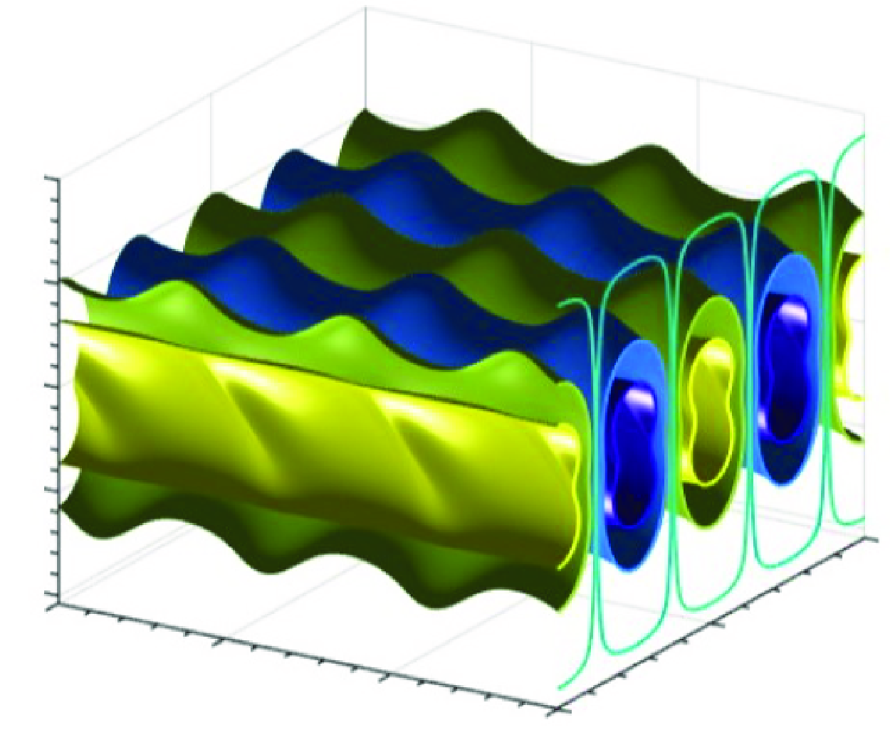
A characteristic flow field topology associated with unstable vortices is illustrated in figure 15. The structure of the disturbance velocity field corresponding to unstable vortices is independent of the wavenumber $\alpha$ (see figures 16 a,b). The centre of the vortex moves closer to the vibrating wall as $Re$ increases, and the disturbance velocity field eventually splits into two layers of vortices, with the primary vortex near the vibrating wall being directly driven by the instability (figures 16 c,d).

Figure 15. Contour plot of the streamwise disturbance velocity component $u_{D}$ for the wave amplitude $A=0.08$ , wavenumber $\alpha =0.7$ , wave speed $c=500$ , flow Reynolds number $Re=1000$ , and vortex wavenumber $\mu =0.7$ .

Figure 16. Distributions of mode zero $g_{u}^{(0)}$ of the x-component of the disturbance velocity vector, and variations of locations of their maxima, as functions of (a,b) the wavenumber $\alpha$ , and (c,d) the Reynolds number $Re$ . All results are for the vortex wavenumber $\mu =0.7$ and the wave amplitude $A=0.08$ .

Finally, we point out that the vortices‘ streaks are susceptible to instabilities (Park, Hwang & Cossu Reference Park, Hwang and Cossu2011). If these occur, then they may lead to either optimal roll structures that maximise the transient temporal growth of the streaks (Schmid & Henningson Reference Schmid and Henningson2001) or asymptotic growth in the form of normal modes leading to secondary instabilities (Floryan Reference Floryan1991).

6. Energy analysis

Further information concerning the properties of the flow can be gleaned by considering the form of the energy transfer between the base flow and the disturbances. To explore this, we can start with the field equations expressed in terms of primitive variables, i.e.

(6.1a,b) \begin{equation}\frac{\partial \boldsymbol{{V}}}{\partial t}+\boldsymbol{{V}}.{\pmb\nabla} \boldsymbol{{V}}+{\pmb\nabla} p={\pmb\nabla} ^{2}\boldsymbol{{V}},\quad {\pmb\nabla} .\boldsymbol{{V}}=0.\end{equation}

The variables are separated into the basic state plus the disturbances, so that

(6.2a,b) \begin{equation}\boldsymbol{{V}}=\boldsymbol{{V}}_{B}+\boldsymbol{{v}}_{D},\quad p=p_{B}+p_{D}.\end{equation}

Substitution of (6.2) into (6.1) and linearisation show that

(6.3) \begin{equation}\frac{\partial \boldsymbol{{v}}_{D}}{\partial t}+\boldsymbol{{V}}_{B}.{\pmb\nabla} \boldsymbol{{v}}_{D}+\boldsymbol{{v}}_{D}.{\pmb\nabla} \boldsymbol{{V}}_{B}+{\pmb\nabla} p_{D}={\pmb\nabla} ^{2}\boldsymbol{{v}}_{D},\quad {\pmb\nabla} .\boldsymbol{{v}}_{D}=0.\end{equation}

An appropriate mechanical energy functional can be constructed by taking the scalar product of the momentum equation with the disturbance velocity vector. The result is then integrated over a control volume that extends across the channel and over one wavelength in the x- and z-directions. This gives (in index notation)

(6.4) \begin{align}&\int _{-1}^{1}\int _{0}^{\lambda _{z}}\!\int _{0}^{\lambda _{x}}\!\left(\frac{1}{2}\frac{\partial }{\partial t}\left(v_{D,i}v_{D,i}\right)+{v_{D,i}}V_{B,j}\frac{\partial v_{D,i}}{\partial x_{j}}+v_{D,i}v_{D,j}\frac{\partial V_{B,i}}{\partial x_{j}}+v_{D,i}\frac{\partial p_{D}}{\partial x_{i}}\!\right){\rm d}x\, {\rm d}z\, {\rm d}y\nonumber\\&\quad=\int _{-1}^{1}\int _{0}^{\lambda _{z}}\int _{0}^{\lambda _{x}}\left({\pmb\nabla} ^{2}v_{D,i}\right).v_{D,i}\, {\rm d}x\, {\rm d}z\, {\rm d}y.\end{align}

The application of periodicity conditions and Green’s theorem leads to

(6.5) \begin{align}&\lambda _{x}^{-1}\lambda _{z}^{-1}\int _{-1}^{1}\int _{0}^{\lambda _{z}}\int _{0}^{\lambda _{x}}\frac{1}{2}\frac{\partial }{\partial t}\left(v_{D,i}v_{D,i}\right) {\rm d}x {\rm d}z {\rm d}y\nonumber\\&\quad=-\lambda _{x}^{-1}\lambda _{z}^{-1}\int _{-1}^{1}\int _{0}^{\lambda _{z}}\int _{0}^{\lambda _{x}}\frac{\partial v_{D,i}}{\partial x_{j}}\frac{\partial v_{D,i}}{\partial x_{j}}{\rm d}x {\rm d}z {\rm d}y\nonumber\\&\qquad-\lambda _{x}^{-1}\lambda _{z}^{-1}\int _{-1}^{1}\int _{0}^{\lambda _{z}}\int _{0}^{\lambda _{x}}v_{D,i}v_{D,j}\frac{\partial V_{B,i}}{\partial x_{j}}{\rm }x {\rm d}z {\rm d}y\end{align}

where the factor $\lambda _{x}^{-1}\lambda _{z}^{-1}$ is included to demonstrate that all quantities are evaluated per unit length in the x- and z-directions. The first term on the right-hand side of this balance describes dissipation, which is always positive, with the normalisation of the disturbance velocity field chosen to make this integral unity. The normalised energy relation then becomes

(6.6) \begin{align}&\lambda _{x}^{-1}\lambda _{z}^{-1}\int _{-1}^{1}\int _{0}^{\lambda _{z}}\int _{0}^{\lambda _{x}}\frac{1}{2}\frac{\partial }{\partial t}\left(v_{D,i}v_{D,i}\right) \,{\rm d}x\, {\rm d}z\, {\rm d}y\nonumber\\&\quad=-1-\lambda _{x}^{-1}\lambda _{z}^{-1}\int _{-1}^{1}\int _{0}^{\lambda _{z}}\int _{0}^{\lambda _{x}}v_{D,i}v_{D,j}\frac{\partial V_{B,i}}{\partial x_{j}}\,{\rm d}x\, {\rm d}z\, {\rm d}y.\end{align}

The left-hand side ( $I_{kin}$ ) denotes the rate of growth of kinetic energy of disturbances. This energy increases with time if the second term on the right-hand side, which captures the inertial effects ( $I_{\textit{inertia}}$ ), dominates over the dissipation. This occurs when $I_{\textit{inertia}}\lt -1$ . The identification of elements of the base flow responsible for the instability requires an explicit decomposition of the inertial integral so that

(6.7) \begin{align}I_{\textit{inertia}}&=\lambda _{x}^{-1}\lambda _{z}^{-1}\int _{-1}^{1}\int _{0}^{\lambda _{z}}\int _{0}^{\lambda _{x}}\left(u_{D}u_{D}\frac{\partial u_{B}}{\partial x}+u_{D}v_{D}\frac{\partial u_{B}}{\partial y}+v_{D}u_{D}\frac{\partial v_{B}}{\partial x}+v_{D}v_{D}\frac{\partial v_{B}}{\partial y}\right)\nonumber\\&\quad\times {\rm d}x\, {\rm d}z\, {\rm d}y=I_{1}+I_{2}+I_{3}+I_{4}.\end{align}

Integration in the x-direction was divided into two parts to enable easy identification of those contributions ascribed to effects of the downwelling and those corresponding to the upwelling parts of the wave. Some typical results are summarised in table 1. These demonstrate that ${\partial u_{B}}/{\partial y}$ combined with Reynolds stresses is mainly responsible for the energy transfer to the disturbances, with other terms having an almost negligible effect. The upwelling and downwelling parts of the wave contribute similar amounts to the energy transfers. The inertial terms have insufficient strength to overcome dissipation when $c=250$ and $c=750$ , but can do it when $c=500$ . When this happens, the Reynolds stress is responsible for the energy transfer.

Table 1. Elements of the energy integral for $A=0.08,\ Re=1000,\ \alpha =0.7,\ \mu =0.07$ .

A qualitative analysis of the energy transfers aids insight into the flow dynamics. The reference flow dominates the primary state as the vibration-created flow modifications are at least an order of magnitude smaller, as was seen in figure 3. This means that

(6.8a–d) \begin{equation}u_{B}\approx Re\, u_{0}\left(y\right),\quad \frac{\partial u_{B}}{\partial y}\approx \frac{1}{2}\,Re,\quad v_{B}\approx 0,\quad\frac{\partial u_{B}}{\partial x}\approx \frac{\partial v_{B}}{\partial x}\approx \frac{\partial v_{B}}{\partial y}\approx 0.\end{equation}

The disturbance velocity field is dominated by mode zero, as portrayed in figure 13. This means that

(6.9a) \begin{equation}u_{D}(x,y,z)\approx g_{u}^{\langle 0\rangle }(y) {\rm e}^{{\rm i}\mu z}+g_{u}^{\langle 0\rangle }(y) {\rm e}^{-{\rm i}\mu z}=2g_{u}^{\langle 0\rangle }(y) \cos(\mu z),\end{equation}

(6.9b) \begin{equation}v_{D}(x,y,z)\approx g_{v}^{\langle 0\rangle }(y) {\rm e}^{{\rm i}\mu z}+g_{v}^{\langle 0\rangle }(y) {\rm e}^{-{\rm i}\mu z}=2g_{v}^{\langle 0\rangle }(y) \cos(\mu z).\end{equation}

Energy integrals $I_{1}, I_{3}, I_{4}$ can be neglected, and $I_{2}$ can be approximated as

(6.10) \begin{equation}I_{2}=Re\int _{-1}^{1}g_{u}^{\left\langle 0\right\rangle }g_{v}^{\left\langle 0\right\rangle }{\rm d}y.\end{equation}

This integral must be sufficiently negative to enable growth in the disturbance energy. This is possible only if the x- and y-disturbance velocity components are out of phase, which indeed is the case as illustrated in the eigenfunctions displayed in figure 13. The phase difference between $u_{D}$ and $v_{D}$ can be explained with the help of the sketch displayed in figure 17. Vortex motions in the downwash zone have a negative $v_{D}$ that brings high-velocity fluid closer to the lower plate and generates a positive $u_{D}$ . The product $v_{D} u_{D}$ is therefore negative, which is the necessary condition to maintain the instability.

Figure 17. Sketch of the unstable fluid movement.

Experimental verification of the above predictions would be desired. Theoretically, at least, one could create well-controlled surface vibrations using a system of piezoelectric pistons turned on and off in a proper sequence to produce surface waves with the desired wavelength and phase speeds. However, this description is somewhat over-simplistic, for it should be recognised that many practical difficulties are associated with constructing such a system. Practical progress is likely to be slow.

7. Summary

This study shows how vibrations applied to a bounding plate can transform the otherwise linearly stable Couette flow into a form susceptible to instability. Appropriately applied vibrations may reduce flow resistance; supercritical waves, i.e. those faster than the flow, always reduce losses. In contrast, the situation for subcritical waves is somewhat more involved and can be determined only after more careful analysis. The vibrations can also lead to instability, and constitute a mechanism capable of generating a secondary flow that manifests as streamwise vortices. If the physical properties of the vibration waves are tuned properly, then instability may set in at a fluid Reynolds number as small as a few hundred. The instability is driven by centrifugal forces created by the wave-imposed changes in the direction of fluid movement, and the process is operative as long as the vibrations are of sufficient size. The disturbance velocity field is characterised by a streamwise velocity component larger than the wall-normal and spanwise components. The resulting streaks are expected to initiate a travelling wave instability driven by an inviscid mechanism associated with inflection points in the distribution of the spanwise velocity component. Such an instability can ultimately lead to Lagrangian chaos.

Surface vibrations may arise as an uncontrolled effect or be introduced intentionally. The calculations described herein form a basis that may guide how the effects of uncontrolled vibrations may be assessed. Such disturbances have the undesirable property that they may prove capable of initiating processes that eventually lead to a premature transition to turbulence.

The mechanisms described here are inherently somewhat complicated. To enable an appreciation of the processes at play, we have supposed that the imposed surface vibration takes the form of a single Fourier mode. In a practical setting, it would be expected that any boundary perturbation would consist of several components of various wavelengths. One could derive the associated stability properties only by conducting careful calculations replicating the exact vibration profile; this may prove difficult. On the other hand, an investigation into the spectrum of vibrations should facilitate the identification of any waves present that might prove particularly effective in causing instability. Such considerations would also provide a means for selecting possible structures for those vibrations that might prove good candidates for achieving some specified control flow objective; conceivably, this might be to reduce the flow resistance, provide a propulsion effect, or increase the efficacious of fluid mixing. Streamwise vortices are particularly relevant to mixing intensification as they include a component of the transverse transport of scalar quantities.

In summary, the considerations described above constitute some of the first calculations aimed at throwing light on the properties of simple shear flows when modified by surface vibrations. We have seen that the situation is somewhat intricate, and there is much scope for extension into various regimes, such as large-amplitude vibrations and practically-important shear flows. We hope to explore and report on some of these avenues in due course.