2 Sphere complexes

In this section, we assume that M is a compact reducible $3$ -manifold with a nonempty boundary. Additionally, in this section, we assume that we do not have spherical boundary components in order to have a prime decomposition with no $3$ -disk factor ([Reference HempelHem76, Chapter 3, Lemma 3.7]). To study the homological finiteness of $\mathrm {B}{\mathrm {Homeo}}^{\delta }(M, \text {rel }\partial )$ inductively based on the number of prime factors in the prime decomposition of M, we shall first construct a simplicial complex $\mathcal {S}(M)$ on which ${\mathrm {Homeo}}^{\delta }(M, \text {rel }\partial )$ acts simplicially.

Note that the group ${\mathrm {Homeo}}^{\delta }(M, \text {rel }\partial )$ acts on $\mathcal {S}(M)$ simplicially. The complex $\mathcal {S}(M)$ is contractible by Proposition 2.3. Therefore, the homotopy quotient $\mathcal {S}(M)/\!\!/ {\mathrm {Homeo}}^{\delta }(M, \text {rel }\partial )$ is homotopy equivalent to $\mathrm {B}{\mathrm {Homeo}}^{\delta }(M, \text {rel }\partial )$ . The stabilizer of each simplex in $\mathcal {S}(M)$ is the subgroup of ${\mathrm {Homeo}}^{\delta }(M, \text {rel }\partial )$ that fixes a set of essential spheres pointwise so it is isomorphic to the homeomorphism group of a $3$ -manifold whose connected components have fewer prime factors. But one issue is that $\mathcal {S}(M)$ has simplices of arbitrary large dimensions since we allow parallel spheres. To account for this infinite dimensionality, we use the simplicial complex that Hatcher and McCullough defined in [Reference Hatcher and McCulloughHM90, Section 1].

The mapping class group $\text {Mod}(M, \text {rel }\partial )=\pi _0({\mathrm {Homeo}}(M, \text {rel }\partial ))$ acts on $[\mathcal {S}](M)$ simplicially. Because all prime factors have nontrivial boundary components that are fixed by $\text {Mod}(M, \text {rel }\partial )$ , as we shall see in Lemma 6.4 if the action of $\text {Mod}(M, \text {rel }\partial )$ fixes a simplex set-wise, it also fixes it pointwise. The complex $[\mathcal {S}](M)$ is finite-dimensional, and also by Hatcher-McCullough’s theorem ([Reference Hatcher and McCulloughHM90, Proposition 2.2]), the set of the orbits of the action of $\text {Mod}(M, \text {rel }\partial )$ on simplices is also finite.

To briefly recall why this is the case, they use a theorem of Scharlemann (see [Reference BonahonBon83, Appendix A, Lemma A.1]) to find a ‘normal representative of each orbit. Let the prime decomposition of M be given by $P_1\# P_2\#\cdots \#P_r\#(\#^{g}\mathbb {S}^1\times \mathbb {S}^2)$ where g summands are homeomorphic to $\mathbb {S}^1\times \mathbb {S}^2$ . Let B be a punctured $3$ -cell having ordered $r+2g$ boundary components so that M is obtained by gluing $P_i\backslash \text {int}(\mathbb {D}^3)$ to i-th sphere boundaries for $1\leq i\leq r$ and g copies of $\mathbb {S}^2\times [0,1]$ are glued along the remaining $2g$ boundary components (see [Reference BonahonBon83, Appendix A, Lemma A.1] for more details).

Now as Hatcher and McCullough observed in [Reference Hatcher and McCulloughHM90, Proposition 2.2], there are finitely many isotopy classes of essential spheres in B since they are determined by the way they partition the boundary components of B. This observation implies the finiteness of the orbits of the action of $\text {Mod}(M, \text {rel }\partial )$ on simplices of $[\mathcal {S}](M)$ .

The skeletal filtration on $[\mathcal {S}](M)$ induces a filtration on the quotient space

(2) $$ \begin{align} \mathcal{F}_0\subset \mathcal{F}_1\subset \dots \subset \mathcal{F}_n=[\mathcal{S}](M)/\text{Mod}(M, \text{rel }\partial), \end{align} $$

and by Hatcher and McCullough’s observation, the filtration quotients are given by the wedge of a finite number of spheres. The reason that the filtration quotients are spheres is the fact that if the action fixes a simplex set-wise, then it fixes it pointwise. Let $\mathcal {O}_p$ be the set of orbits of the action of $\text {Mod}(M, \text {rel }\partial )$ on p-simplices of $[\mathcal {S}](M)$ . So $\mathcal {F}_p-\mathcal {F}_{p-1}$ is homeomorphic to $\coprod _{\sigma \in \mathcal {O}_p} \dot {\Delta }^p_{\sigma }$ , the disjoint union of open p-simplices indexed by $\mathcal {O}_p$ .

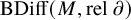
Figure 1 $\sigma $ here is a $2$ -simplex consisting of 3 separating spheres that are drawn in one dimension lower.

The natural simplicial map $\mathcal {S}(M)\to [\mathcal {S}](M)$ that sends spheres to their isotopy classes is equivariant with respect to the map ${\mathrm {Homeo}}^{\delta }(M, \text {rel }\partial )\to \text {Mod}(M, \text {rel }\partial )$ . So we have a map $\mathcal {S}(M)/{\mathrm {Homeo}}^{\delta }(M, \text {rel }\partial )\to [\mathcal {S}](M)/\text {Mod}(M, \text {rel }\partial )$ which in turn induces a map

$$\begin{align*}\eta\colon \mathcal{S}(M)/\!\!/ {\mathrm{Homeo}}^{\delta}(M, \text{rel }\partial)\to [\mathcal{S}](M)/\text{Mod}(M, \text{rel }\partial). \end{align*}$$

We are interested in local coefficient systems that are pullbacks of local coefficients systems on $\mathrm {B}{\mathrm {Homeo}}(M, \text {rel }\partial )$ . Since we have the maps

$$\begin{align*}\mathcal{S}(M)/\!\!/ {\mathrm{Homeo}}^{\delta}(M, \text{rel }\partial)\to \mathrm{B}{\mathrm{Homeo}}^{\delta}(M, \text{rel }\partial)\to \mathrm{B}{\mathrm{Homeo}}(M, \text{rel }\partial), \end{align*}$$

for each point x in the image of $\eta $ , we have a map $\eta ^{-1}(x)\to \mathrm {B}{\mathrm {Homeo}}(M, \text {rel }\partial )$ that is uniquely determined up to homotopy. It turns out, as we shall see, that the restriction of $\eta $ to each open simplex $\dot {\Delta }^p_{\sigma }$ is a fiber bundle (see Section 5) whose fiber, by an inductive argument, is $\mathcal {L}$ -homologically finite for all $\mathcal {L}$ that are pullbacks from local coefficient systems on $\mathrm {B}{\mathrm {Homeo}}(M, \text {rel }\partial )$ .

Then the weak homological finiteness of $\mathrm {B}{\mathrm {Homeo}}^{\delta }(M, \text {rel }\partial )$ will follow from a general statement about simplicial complexes where in this generality, to clarify the original argument, was suggested to the author by the referee.

The simplicial map $ \mathcal {S}(M)\to [\mathcal {S}](M)$ is ${\mathrm {Homeo}}^{\delta }(M, \text {rel }\partial )$ -equivariant, and we already know that the conditions (1) and (3) are satisfied. So Theorem 1.1 follows from Lemma 2.9 and Theorem 2.8. The bulk of the work is to prove Theorem 2.8, and we shall prove Lemma 2.9 in Section 5.

In Section 6 and Section 7, we find a model for $\eta ^{-1}(x)$ to which we can apply the induction hypothesis, the strong homological finiteness of $\mathrm {B}{\mathrm {Homeo}}(M, \text {rel }\partial )$ for M with fewer prime factors) when M is connected sum of irreducible factors that each have a nontrivial boundary.

3 Reformulation of the main theorem and an inductive strategy

In this section, we shall use the hypothesis that the prime decomposition of M consists of irreducible factors that each have nonempty non-spherical boundary components. We choose a base point on the boundary of M. We denote this boundary component by $\partial _*M$ . The goal is for each p and each $x\in \mathcal {F}_p-\mathcal {F}_{p-1}$ to find a semi-simplicial space $X_{\bullet }$ whose realization admits an acyclic map from $\eta ^{-1}(x)$ and sits in a fibration sequence so that by induction on the number of prime factors, we could argue that the fiber and the base are weakly homologically finite with compatible maps.

The advantage of working with $ 3$ -manifolds that are connected sums of irreducible pieces such that each have a nonempty boundary is the following:

• • When we cut along essential separating spheres, the remaining pieces each have a non-spherical boundary component that is fixed, and we shall use this for the inductive argument.

• • Since each irreducible factor has a nontrivial boundary that is fixed, homeomorphic irreducible factors cannot be permuted under the action of ${\mathrm {Homeo}}(M, \text {rel }\partial )$ .

To be able to induct on the number of prime factors of M, we shall prove a slightly more general statement of Theorem 1.1 taking into account spherical boundary components.

Recall that the corresponding automorphism groups in $C^0$ -category and $C^{\infty }$ -category are weakly homotopy equivalent.

Cerf ([Reference CerfCer61]) assumed Smale’s conjecture which was later proved by Hatcher ([Reference HatcherHat83]) to show that in these low dimensions, the inclusion $\mathrm {Diff}(M)\hookrightarrow \mathrm {Homeo}(M)$ is a weak homotopy equivalence. So to prove our homological finiteness result, we freely use diffeomorphism groups and homeomorphism groups depending on the convenience of the situation.

Let $e_i\colon \mathbb {D}^3\hookrightarrow M$ for $1\leq i\leq k+l$ be disjoint embeddings, and let N be the $3$ -manifold obtained from M by removing $e_i(\text {int}(\mathbb {D}^3))$ for all $1\leq i\leq k+l$ . So the boundary of N is the union of $\partial M$ with sphere boundary components, which we denote by $S_i$ . We denote the union of the sphere boundary components $ \{S_i\}_{i=1}^k$ by $S_{\text {free}}$ and union of the rest of the sphere boundary components by $S_{\text {fixed}}$ . Let ${\mathrm {Homeo}}(N, S_{\text {free}}, \text {rel }(\partial M\cup S_{\text {fixed}}))$ be the subgroup of ${\mathrm {Homeo}}(N, \text {rel }(\partial M\cup S_{\text {fixed}}))$ whose elements fix each sphere in $S_{\text {free}}$ set-wise.

Theorem 1.1 is a special case of Theorem 3.2. But as we shall see in Section 4, in fact, they are equivalent statements. However, the statement of Theorem 3.2 is more convenient for the inductive argument.

Our first goal is to use Theorem 3.2 inductively for fewer prime factors than the number of prime factors of M to show that for each p and each $x\in \mathcal {F}_p-\mathcal {F}_{p-1}$ , the pre-image $\eta ^{-1}(x)$ is weakly homologically finite. To fix ideas, let x be in $\mathcal {F}_0$ in the filtration 2 which is the image of a separating sphere $S\subset M$ . This is because all vertices in $\mathcal {S}(M)$ are separating since the prime decomposition of M does not have $\mathbb {S}^1\times \mathbb {S}^2$ summands.

Suppose that the sphere S cuts the manifold M into two pieces $M_1$ and $M_2$ where $M_1$ contains $\partial _* M$ , the boundary component of M with the base point. Let ${\mathrm {Homeo}}(M_1, S, \text {rel }\partial M)$ be the subgroup of ${\mathrm {Homeo}}(M_1)$ that fixes the boundary component S set-wise and the rest of the boundary components pointwise. In Section 6, we shall prove that there is an acyclic map from $\eta ^{-1}(x)$ to the realization of a semi-simplicial space (in fact a two-sided bar construction) $X_{\bullet }$ that fits in a homotopy fiber sequence

(3) $$ \begin{align} \mathrm{B}{\mathrm{Homeo}}(M_2, \text{rel }\partial)\to ||X_{\bullet}||\to \mathrm{B}{\mathrm{Homeo}}(M_1, S, \text{rel }\partial M). \end{align} $$

Note that $M_1$ and $M_2$ have sphere boundary components. When we fill in those sphere boundary components with balls, they have fewer prime factors compared to M. By the induction hypothesis, Theorem 3.2 implies that the fiber $\mathrm {B}{\mathrm {Homeo}}(M_2, \text {rel }\partial )$ and the base $\mathrm {B}{\mathrm {Homeo}}(M_1, S, \text {rel }\partial M)$ are strongly homologically finite. Then the following lemma implies that $||X_{\bullet }||$ is also strongly homologically finite.

It will be by construction that the map $\eta ^{-1}(x)\to \mathrm {B}{\mathrm {Homeo}}(M, \text {rel }\partial )$ factors through the map $\eta ^{-1}(x)\to ||X_{\bullet }||$ . Therefore, in this way, we shall deduce that $\eta ^{-1}(x)$ is a weakly homologically finite space by induction on the number of prime factors, and then Theorem 3.2 will follow from Lemma 2.9. First, let us settle the induction’s base case for Theorem 3.2.

4 The base case of induction and spherical boundary components

In this section, we shall see that Theorem 1.1 and Theorem 3.2 are equivalent, and we prove Theorem 4.1 that is stronger than the base case of Theorem 3.2.

Let P be an irreducible $ 3$ -manifold with a nonempty and non-spherical boundary. Let $e_i\colon \mathbb {D}^3\hookrightarrow P$ for $1\leq i\leq k+l$ be disjoint embeddings, and let N be the $3$ -manifold obtained from P by removing $e_i(\text {int}(\mathbb {D}^3))$ for all $1\leq i\leq k+l$ . So the boundary of N is the union of $\partial P$ with sphere boundary components, which we denote by $S_i$ . We denote the union of the sphere boundary components $ \{S_i\}_{i=1}^k$ by $S_{\text {free}}$ and union of the rest of the sphere boundary components by $S_{\text {fixed}}$ . The group ${\mathrm {Homeo}}(N, \text {rel }(\partial P\cup S_{\text {fixed}}))$ fixes the boundary components $S_{\text {free}}$ set-wise. To keep track of free spherical boundary components, in what follows, we also add $S_{\text {free}}$ to the notation ${\mathrm {Homeo}}(N, \text {rel }(\partial P\cup S_{\text {fixed}}))$ (e.g., ${\mathrm {Homeo}}(N, S_{\text {free}}, \text {rel }(\partial P\cup S_{\text {fixed}}))$ without having “rel” before the free boundary components).

This, of course, implies the base case of Theorem 3.2. Since the corresponding diffeomorphism groups and homeomorphism groups are weakly equivalent (by Theorem 3.1), we shall instead prove that $\mathrm {BDiff}(N, S_{\text {free}}, \text {rel }\partial P\cup S_{\text {fixed}})$ has a finite CW complex model.

We already know the homotopical finiteness for an irreducible $3$ -manifold with a nonempty boundary ([Reference Hatcher and McCulloughHM97]).

So we know that $\mathrm {BDiff}(P, \text {rel }\partial )$ has a finite CW complex model. We want to inductively fix $e_i(\mathbb {D}^3)$ either set-wise or pointwise and still get a finite CW complex model.

Proof. Including the diffeomorphism group that fixes a neighborhood of the boundary into the diffeomorphism group that fixes the boundary pointwise is a weak homotopy equivalence (see [Reference KupersKup19a, Chapter 4 and 5]). So let $\mathrm {Diff}(P, S_{\text {free}}, \text {fix }e(D^3), \text {rel }\partial _1)$ be the subgroup of $\mathrm {Diff}(P, S_{\text {free}}, \text {rel }\partial _1)$ that fixes $e(D^3)$ pointwise. The inclusion

$$\begin{align*}\mathrm{Diff}(P, S_{\text{free}}, \text{rel }\partial_1 \cup e(D^3))\to \mathrm{Diff}(P, S_{\text{free}}, \text{fix }e(D^3), \text{rel }\partial_1), \end{align*}$$

is a weak homotopy equivalence. Hence, using [Reference PalaisPal60, Theorem C] and the above weak equivalence, we have a homotopy fiber sequence

$$\begin{align*}\mathrm{Diff}(P, S_{\text{free}}, \text{rel }\partial_1 \cup e(D^3))\to \mathrm{Diff}(P, S_{\text{free}}, \text{rel }\partial_1)\to \text{Emb}^+(D^3, P)\simeq \text{Fr}^+(P), \end{align*}$$

where $\text {Emb}^+(D^3, P)$ is the space of orientation preserving embeddings and $\text {Fr}^+(P)$ is the oriented frame bundle of M. It can be delooped (similar to the standard fact [Reference Félix, Oprea and TanréFOT08, Proposition 1.80]) to induce the fiber sequence

$$\begin{align*}\text{Fr}^+(P)\to \mathrm{BDiff}(P, S_{\text{free}}, \text{rel }\partial_1 \cup e(D^3))\to \mathrm{BDiff}(P, S_{\text{free}}, \text{rel }\partial_1). \end{align*}$$

The base and the fiber of this fiber sequence have the homotopy type of a finite CW-complex (strongly homologically finite). Therefore, the total space also has a finite CW-complex model (strongly homologically finite).

Proof. For simplicity, we consider the case where P is closed; the general case follows similarly. Let $\mathrm {Diff}(M, \text {rel } \partial _{\text {SO}(3)})$ be the subgroup of $\mathrm {Diff}(M)$ that on a neighborhood of the boundary S restricts to the subgroup of rigid rotations in the following sense. We fix a collar neighborhood $e\colon S^2\times [0,1)\hookrightarrow M$ extending the parametrization of the boundary S. The group of rotations $\text {SO}(3)$ acts on this collar neighborhood by acting on each slice $e(S^2\times \{t\})$ by a fixed rotation. For each element f of $\mathrm {Diff}(M, \text {rel } \partial _{\text {SO}(3)})$ , there exists a positive $\epsilon $ such that the restriction of f to $e(S^2\times [0,\epsilon ))$ is the same as the action of $\text {SO}(3)$ . Recall that Smale’s theorem ([Reference SmaleSma59]) implies that $\mathrm {Diff}_0(S^2)\simeq \text {SO}(3)$ . Hence, by the comparison of fiber sequences, it is easy to see that $\mathrm {Diff}(M, \text {rel } \partial _{\text {SO}(3)})$ is homotopy equivalent to $\mathrm {Diff}(M)$ .

So it is enough to show that the natural inclusion

$$\begin{align*}\mathrm{Diff}(M, \text{rel } \partial_{\text{SO}(3)})\to \mathrm{Diff}(P, x), \end{align*}$$

that is induced by extending a rotation on the boundary of $e(D^3)$ to its interior, is a homotopy equivalence.

Recall that Hatcher’s theorem implies that $\mathrm {Diff}(D^3, \text {rel }S^2)$ is contractible which in turn implies that the restriction map $\mathrm {Diff}(D^3)\to \mathrm {Diff}(S^2)$ is a homotopy equivalence. Let $\mathrm {Diff}(P, e(D^3))$ be the subgroup of $\mathrm {Diff}(P)$ that fixes $e(D^3)$ set-wise. Since $\mathrm {Diff}^+(D^3)\simeq \text {SO}(3)$ , by the comparison of fibrations, one can see that the inclusion $\mathrm {Diff}(M, \text {rel } \partial _{\text {SO}(3)})\to \mathrm {Diff}(P, e(D^3))$ is a homotopy equivalence.

However, since $D^3$ is contractible, the fiber sequence obtained by the action of $\mathrm {Diff}^+(D^3)$ on $D^3$ implies that the inclusion $\mathrm {Diff}^+(D^3, 0)\hookrightarrow \mathrm {Diff}^+(D^3)$ is a weak equivalence where $\mathrm {Diff}^+(D^3, 0)$ is the subgroup fixing the origin of $D^3$ . Let $\mathrm {Diff}(P, e(D^3), x)$ be the subgroup of $\mathrm {Diff}(P, e(D^3))$ that fixes the point x. By comparison of fiber sequences, one can see that $\mathrm {Diff}(P, e(D^3), x)\to \mathrm {Diff}(P, e(D^3))$ is also a weak equivalence. Therefore, it is enough to show that $\mathrm {Diff}(P, e(D^3), x)\to \mathrm {Diff}(P,x)$ is a weak equivalence. Consider the following fiber sequence that is a variant of the fiber sequence [Reference PalaisPal60, Theorem C]

$$\begin{align*}\mathrm{Diff}(P, e(D^3), x)\to \mathrm{Diff}(P, x)\to \text{Emb}^+((D^3,0), (P, x))/\mathrm{Diff}(D^3,0), \end{align*}$$

where $\text {Emb}^+((D^3,0), (P, x))/\mathrm {Diff}(D^3,0)$ is the space of unparametrized smooth embeddings of $D^3$ that send its center to x. It is easy to see that $\text {Emb}^+((D^3,0), (P, x))/\mathrm {Diff}(D^3,0)$ is contractible. Hence, $\mathrm {Diff}(P, e(D^3), x)\to \mathrm {Diff}(P, x)$ is a weak equivalence.

Proof of Theorem 4.1.

We shall prove that $\mathrm {BDiff}(N, S_{\text {free}}, \text {rel }(\partial P\cup S_{\text {fixed}}))$ has a finite CW complex model. Let M be the manifold obtained from P by removing $e_i(\text {int}(\mathbb {D}^3))$ for all $1\leq i\leq k$ . Given Lemma 4.3, it is enough to prove that $\mathrm {BDiff}(M, S_{\text {free}}, \text {rel }\partial P)$ has a finite CW complex model.

Let $x_i$ be a point in P given by the image of the center of the ball $e_i(\text {int}(\mathbb {D}^3))$ . Let $\mathrm {Diff}(P, \{x_1,\dots ,x_k\}, \text {rel }\partial P)$ be the subgroup of $\mathrm {Diff}(P, \text {rel }\partial P)$ consisting of those elements that fix each $x_i$ .

Claim. The classifying space $\mathrm {BDiff}(M, S_{\text {free}}, \text {rel }\partial P)$ is homotopy equivalent to $\mathrm {BDiff}(P, \{x_1,\dots ,x_k\}, \text {rel }\partial P)$ .

This is easily deduced by applying Lemma 4.4 inductively k times.

Let $\text {PConf}_k(P)$ be the space of ordered configuration space of k points in the interior of P. Forgetting the first point induces the map

$$\begin{align*}\text{PConf}_k(P)\to \text{PConf}_{k-1}(P), \end{align*}$$

which is a fibration whose fiber is homotopy equivalent to the complement of $(k-1)$ points in P. Hence, inductively we conclude that $\text {PConf}_k(P)$ is weakly equivalent to a finite CW complex. Considering the action of $\mathrm {Diff}(P, \text {rel }\partial P)$ on the k points $\{x_1,\dots ,x_k\}$ gives a Palais fiber sequence ([Reference PalaisPal60, Theorem C]). By delooping this fiber sequence, we have a fiber sequence

$$\begin{align*}\text{PConf}_k(P)\to \mathrm{BDiff}(P,\{x_1,\dots,x_k\}, \text{rel }\partial P)\to \mathrm{BDiff}(P, \text{rel }\partial P). \end{align*}$$

Since both $\mathrm {BDiff}(P, \text {rel }\partial P)$ and $\text {PConf}_k(P)$ have a finite CW complex model, so does $ \mathrm {BDiff}(P,\{x_1,\dots ,x_k\}, \text {rel }\partial P)$ .

Note that the proof of Lemma 4.4 and the proof of the claim above imply that if $\mathrm {BDiff}(M, \text {rel }\partial )$ is homologically finite, so is $\mathrm {BDiff}(N, S_{\text {free}}, \text {rel }(\partial P\cup S_{\text {fixed}}))$ . Therefore, Theorem 3.2 is also implied by Theorem 1.1.

5 Proof of the technical Lemma 2.9

We denote the image of a simplex $\Delta \subset Y$ in $Y/G$ by $[\Delta ]$ . Because of conditions (2) and (3), the cells $[\Delta ]$ give a finite CW structure on $Y/G$ and let S be the finite set of all cells.

Step $\mathbf {0}$ : For a simplex $\Delta \subset Y$ , let $X(\Delta )$ be the subcomplex of X that is the preimage of $\Delta $ under the map $X\to Y$ . Then it is well known ([Reference Kirby and SiebenmannKS77, Lemma 1.7 in Essay III at page 94]) that the restriction of $X(\Delta )\to \Delta $ to the interior $\dot {\Delta }$ is a trivial fiber bundle. A more streamlined proof is given in [Reference WilliamsonWil66, Theorem 1.3.1]. Note that the finiteness condition in [Reference WilliamsonWil66, Reference Kirby and SiebenmannKS77] is used in the second half of their proof where they want to prove it is a PL fiber bundle. To prove that topologically this restriction is a trivial fiber bundle as they showed, the finiteness condition on $X(\Delta )$ is not needed.

Step $\mathbf {1}$ : Let $[\dot {\Delta }_{\alpha }]$ be the interior of the cell $[\Delta _{\alpha }]$ for $\alpha \in S$ . We shall prove that for each cell $[\Delta _{\alpha }]$ , the restriction of $\eta $ to the interior $[\dot {\Delta }_{\alpha }]$ is a trivial fiber bundle.

Let $X([\Delta _{\alpha }])\subset X$ be the subcomplex that is the pre-image of $[\Delta _{\alpha }]$ under the map g that is the composition $g\colon X\to Y\to Y/G$ , and let $X([\dot {\Delta }_{\alpha }])$ be the preimage of $[\dot {\Delta }_{\alpha }]$ . So we want to show that the map

$$\begin{align*}X([\dot{\Delta}_{\alpha}])/\!\!/ G\to [\dot{\Delta}_{\alpha}] \end{align*}$$

is a trivial fiber bundle. Since the map $X\to Y$ is G-equivariant, the map

$$ \begin{align*}X([\dot{\Delta}_{\alpha}])\to \text{orbit}(\dot{\Delta}_{\alpha})\end{align*} $$

is also a trivial fiber bundle by step $0$ where $\text {orbit}(\dot {\Delta }_{\alpha })$ is the orbit of $\dot {\Delta }_{\alpha }$ under the G action. Let $b_{\alpha }$ be the barycenter of $[\dot {\Delta }_{\alpha }]$ . So there is a natural homeomorphism $X([\dot {\Delta }_{\alpha }])\cong [\dot {\Delta }_{\alpha }]\times g^{-1}(b_{\alpha })$ which is G-equivariant where G-action on $[\dot {\Delta }_{\alpha }]$ is trivial and on $X([\dot {\Delta }_{\alpha }])$ and $g^{-1}(b_{\alpha })$ are the natural actions restricted from the action on X. Hence, we obtain a natural homeomorphism

$$\begin{align*}X([\dot{\Delta}_{\alpha}])/\!\!/ G\cong [\dot{\Delta}_{\alpha}]\times (g^{-1}(b_{\alpha})/\!\!/ G) \end{align*}$$

that commutes with the projection to $ [\dot {\Delta }_{\alpha }]$ .

Step 2: Since the inclusion of sub-CW-complexes are cofibrations, there is an open neighborhood U of each sub-CW-complex K in $Y/G$ that deformation retracts to K. But we also want U to satisfy the following property. Let $Y(K)$ be the G-invariant sub-simplicial-complex of Y that is the preimage of K via the quotient map $Y\to Y/G$ , and let $Y(U)$ be a G-invariant open neighborhood of $Y(K)$ in the preimage of U in Y. Similarly, we have G-invariant subspaces $X(K)$ and $X(U)$ . Since the map $X\to Y$ is simplicial, we want to choose U small enough so that $X(U)$ deformation retracts to $X(K)$ .

To fix such a neighborhood U, we can choose it combinatorially (one can also do it by putting metrics on Y and X). Barycentrically subdivide Y twice and choose the regular neighborhood U of K. The simplicial map $f\colon X\to Y$ can be realized as the realization of the poset map between barycentric subdivisions. So then, one can see that similar to the canonical deformation retraction of U to K that is done simplex by simplex, $X(U)$ also deformation retracts to $X(K)$ .

Since the preimage $\eta ^{-1}(U)$ is $X(U)/\!\!/ G$ , and the map $X(K)\to X(U)$ is G-equivariant, we deduce that the inclusion $\eta ^{-1}(K)\hookrightarrow \eta ^{-1}(U)$ is a weak homotopy equivalence. We can inductively apply Mayer-Vietoris as follows.

Step 3: By induction on the dimension of the sub-CW-complex K, suppose we know that $\eta ^{-1}(K)$ is $\mathcal {L}|_{\eta ^{-1}(K)}$ -homologically finite for $\text {dim}(K)<k$ . The base of the induction is guaranteed by condition (2). Now we consider the sub-CW complex $K\cup _{ [\partial \Delta _\alpha ]} [\Delta _\alpha ]$ . Let the open neighborhood U of K be as in step $2$ . So it is enough to show that $\eta ^{-1}(U\cup [\dot {\Delta }_{\alpha }])$ is $\mathcal {L}|_{\eta ^{-1}(U\cup [\dot {\Delta }_{\alpha }])}$ -homologically finite. Note that this space is covered by open sets $\eta ^{-1}(U)$ and $\eta ^{-1}( [\dot {\Delta }_{\alpha }])$ whose intersection is the preimage of $ [\dot {\Delta }_{\alpha }]\cap U$ . We can choose U so that as in step $2$ , the preimage $\eta ^{-1}([\dot {\Delta }_{\alpha }]\cap U)$ is homeomorphic to $ ([\dot {\Delta }_{\alpha }]\cap U)\times (g^{-1}(b_{\alpha })/\!\!/ G)$ . So $\eta ^{-1}([\dot {\Delta }_{\alpha }]\cap U)$ is also $\mathcal {L}|_{\eta ^{-1}([\dot {\Delta }_{\alpha }]\cap U)}$ -homologically finite.

By induction, we know that $\eta ^{-1}(U)$ is $\mathcal {L}|_{\eta ^{-1}(U)}$ -homologically finite. Step $1$ and condition (2) imply that $\eta ^{-1}( [\dot {\Delta }_{\alpha }])$ is of $\mathcal {L}|_{\eta ^{-1}( [\dot {\Delta }_{\alpha }])}$ -homologically finite. Therefore, Mayer-Vietoris with local coefficient systems ([Reference WhiteheadWhi12, Chapter VI]) implies the same for the preimage of $K\cup _{\partial [\Delta _\alpha ]} [\Delta _\alpha ]$ . Given that $Y/G$ is a finite complex, this process of adding cells ends in a finite step which implies that $X/\!\!/ G$ is $\mathcal {L}$ -homologically finite.

6 The homological finiteness of $\eta ^{-1}(x)$ for a vertex x

Let x be in $\mathcal {F}_0$ in the filtration 2 which is the image of a separating sphere $S\subset M$ . Our first step to identify the homotopy type of $\eta ^{-1}(x)$ is the following proposition. Let $\mathcal {S}(M, [S])$ be the full subcomplex of $\mathcal {S}(M)$ whose vertices are the orbits of S under the action of ${\mathrm {Homeo}}^{\delta }(M, \text {rel }\partial )$ .

Proposition 6.1. Let x be in $\mathcal {F}_0$ . The preimage $\eta ^{-1}(x)$ is homotopy equivalent to

$$\begin{align*}\mathcal{S}(M, [S])/\!\!/ {\mathrm{Homeo}}^{\delta}(M, \text{rel }\partial). \end{align*}$$

Before proving Proposition 6.1, let us first observe some properties of the subcomplex $\mathcal {S}(M, [S])$ . Note that in a simplex, there could be vertices that are given by isotopic spheres, and since they are disjoint, at least for M satisfying the hypothesis of Theorem 3.2, they bound an embedded $\mathbb {S}^2\times [0,1]$ . By Scharlemann’s theorem, we can send two disjoint spheres $S_1$ and $S_2$ by a homeomorphism into B. Since the isotopy classes of embedded spheres in B are determined by how an embedded sphere separates the boundary components (see [Reference Hatcher and McCulloughHM90, Proposition 2.2]), two disjoint isotopic spheres in B bound a $\mathbb {S}^2\times [0,1]$ . Now if the image of $S_1$ and $S_2$ in B are not isotopic in B, then they separate disjoint diffeomorphic submanifolds of M in which case, given that each irreducible factor has a nontrivial boundary, the spheres $S_i$ could not be isotopic in M relative to the boundary. So we record this fact as a lemma.

Proof of Proposition 6.1.

Let $x\in \mathcal {F}_0$ be an orbit of an isotopy class $[S]$ of a separating sphere S. Let $[\mathcal {S}](M, [S])$ be the full subcomplex of $[\mathcal {S}](M)$ whose vertices are the orbits of $[S]$ . Consider the commutative diagram

(4)

The preimage of x in $\mathcal {S}(M)$ is the subcomplex $\mathcal {S}(M, [S])$ which is ${\mathrm {Homeo}}^{\delta }(M, \text {rel }\partial )$ -invariant. So $\eta _1^{-1}(x)$ is the quotient space $\mathcal {S}(M, [S])/{\mathrm {Homeo}}^{\delta }(M, \text {rel }\partial )$ . Now by the naturality of the Borel construction, we have a pullback diagram

(5)

Hence, the preimage $\eta ^{-1}(x)=\eta _2^{-1}(\mathcal {S}(M, [S])/{\mathrm {Homeo}}^{\delta }(M, \text {rel }\partial ))$ is in fact homeomorphic to the Borel construction $\mathcal {S}(M, [S])/\!\!/{\mathrm {Homeo}}^{\delta }(M, \text {rel }\partial )$ .

Now we define a semi-simplicial space whose underlying semi-simplicial set is $\mathcal {S}_{\bullet }(M, [S])$ .

For a p-simplex $e_p\in \mathcal {S}^{\tau }_{p}(M, [S])$ , let $\text {Stab}(e_p)$ be the subgroup of ${\mathrm {Homeo}}(M, \text {rel }\partial )$ that fixes $e_p$ pointwise. By Lemma 6.2 and Lemma 6.4, each p-simplex is given by $p+1$ parallel spheres. Let $\sigma _1=(S_0, S_1, \dots , S_p)$ and $\sigma _2=(S_0', S_1', \dots , S_p')$ be two p-simplices where the order of the spheres are induced by the inside to outside order. Since the action of ${\mathrm {Homeo}}^{\delta }(M, \text {rel }\partial )$ on the set $\mathcal {S}_{0}(M, [S])$ is transitive, we can find $f_0\in {\mathrm {Homeo}}^{\delta }(M, \text {rel }\partial )$ such that $f_0(S_0')=S_0$ . Note that $f_0(S_1')$ is isotopic to $S_1$ and they are disjoint from $S_0$ . So by the isotopy extension theorem ([Reference Edwards and KirbyEK71, Corollary 1.2]), there exists $f_1\in {\mathrm {Homeo}}^{\delta }_0(M, \text {rel }\partial )$ whose support does not intersect $S_0$ and $f_1(S_1')=S_1$ . Continuing this process, we can find $f_i\in {\mathrm {Homeo}}^{\delta }_0(M, \text {rel }\partial )$ for $1\leq i\leq p$ such that $f_p\circ \dots \circ f_0$ sends $S_i'$ to $S_i$ for all $0\leq i\leq p$ . Therefore, the action of ${\mathrm {Homeo}}^{\delta }(M, \text {rel }\partial )$ on the set of p-simplices is transitive. Hence, the topological version of Shapiro’s lemma implies that there is a map $\mathrm {B}\text {Stab}^{\delta }(e_p)\to \mathcal {S}_{p}(M, [S])/\!\!/ {\mathrm {Homeo}}^{\delta }(M, \text {rel }\partial )$ that is a weak equivalence. To show that the homotopy quotient $\mathcal {S}^{\tau }_{p}(M, [S])/\!\!/ {\mathrm {Homeo}}(M, \text {rel }\partial )$ is homotopy equivalent to $\mathrm {B}\text {Stab}(e_p)$ , we need the following lemma. Let $\text {Sing}_{\bullet }(X)$ denote the singular set of a topological space X. Recall that by [Reference MilnorMil57] and [Reference Ebert and Randal-WilliamsERW19, Lemma 1.7], the augmentation map $ \text {Sing}_{\bullet }(X)\to X$ induces a weak equivalence after fat realization.

Proof. Let $\mathcal {S}^{\tau }_{p}(M, [S])_{\bullet }$ be defined similarly to $\mathcal {S}^{\tau }_{p}(M, [S])$ in Definition 6.6, but instead of the space of locally flat embeddings, we consider the simplicial set of locally flat embeddings $\text {Emb}^{\mathsf {{lf}}}(\mathbb {S}^2, M)_{\bullet }$ (see [Reference NarimanNar20, Definition 2.5]). Then the action of ${\mathrm {Homeo}}(M, \text {rel }\partial )$ on $\mathcal {S}^{\tau }_{p}(M, [S])$ induces the following map of simplicial sets

$$\begin{align*}\text{Sing}_{\bullet}({\mathrm{Homeo}}(M, \text{rel }\partial))\to \mathcal{S}^{\tau}_{p}(M, [S])_{\bullet}, \end{align*}$$

which by the parametrized isotopy extension theorem, it is a Kan fibration (see [Reference Burghelea and LashofBL74, Page 19] where it is called A.I.T which is short for the ambient isotopy extension theorem) whose fiber is $\text {Sing}_{\bullet }(\text {Stab}(e_p))$ .

Again, the augmentation map $\mathcal {S}^{\tau }_{p}(M, [S])_{\bullet }\to \mathcal {S}^{\tau }_{p}(M, [S])$ induces a weak equivalence after fat realization, and it is equivariant with respect to the map $\text {Sing}_{\bullet }({\mathrm {Homeo}}(M, \text {rel }\partial ))\to {\mathrm {Homeo}}(M, \text {rel }\partial )$ . So we obtain a natural weak equivalence

$$\begin{align*}||\mathcal{S}^{\tau}_{p}(M, [S])_{\bullet}/\!\!/ \text{Sing}_{\bullet}({\mathrm{Homeo}}(M, \text{rel }\partial))||\xrightarrow{\simeq}\mathcal{S}^{\tau}_{p}(M, [S])/\!\!/ {\mathrm{Homeo}}(M, \text{rel }\partial). \end{align*}$$

Therefore, it is enough to show that for each k in the simplicial direction, we have a map

$$\begin{align*}\mathrm{B}\mathrm{Sing}_{k}(\text{Stab}(e_p))\to \mathcal{S}^{\tau}_{p}(M, [S])_{k}/\!\!/ \text{Sing}_{k}({\mathrm{Homeo}}(M, \text{rel }\partial)), \end{align*}$$

that induces a weak equivalence.

Let G be the discrete group $\text {Sing}_{k}({\mathrm {Homeo}}(M, \text {rel }\partial ))$ , and let H be its subgroup $\mathrm {Sing}_{k}(\text {Stab}(e_p))$ . Note that there is natural isomorphism from the coset $G/H$ to $\mathcal {S}^{\tau }_{p}(M, [S])_{k}$ . As is also mentioned in [Reference NarimanNar20, Section 3.1.1], the Shapiro’s lemma for discrete groups implies that there is a natural map $\mathrm {B}H\to (G/H)/\!\!/ G$ which is a weak homotopy equivalence.

Now note that Thurston’s homology isomorphism 1, in the generality that McDuff proved in [Reference McDuffMcD80, Section 2], implies that the map

$$\begin{align*}\mathrm{B}\text{Stab}^{\delta}(e_p)\to \mathrm{B}\text{Stab}(e_p) \end{align*}$$

is an acyclic map. This map factors through $\mathrm {B}\text {Stab}^{\delta }(e_p)\to \mathrm {B}|\mathrm {Sing}_{\bullet }(\text {Stab}(e_p))|$ which is induced by mapping $\text {Stab}^{\delta }(e_p)$ to the $0$ -simplices $\mathrm {Sing}_{0}(\text {Stab}(e_p))$ . So using Lemma 6.7, we obtain that for each p, the natural map

(6) $$ \begin{align} f_p\colon\mathcal{S}_{p}(M, [S])/\!\!/ {\mathrm{Homeo}}^{\delta}(M, \text{rel }\partial)\to \mathcal{S}^{\tau}_{p}(M, [S])/\!\!/ {\mathrm{Homeo}}(M, \text{rel }\partial) \end{align} $$

induces an acyclic map. We claim that the induced map between the realizations

$$\begin{align*}f\colon ||\mathcal{S}_{\bullet}(M, [S])/\!\!/ {\mathrm{Homeo}}^{\delta}(M, \text{rel }\partial)||\to ||\mathcal{S}^{\tau}_{\bullet}(M, [S])/\!\!/ {\mathrm{Homeo}}(M, \text{rel }\partial)|| \end{align*}$$

is also acyclic. Because for a local coefficient $\mathcal {L}$ on the realization $||X_{\bullet }||$ of a semisimplicial space $X_{\bullet }$ , there is a spectral sequence that calculates the homology of the realization with local coefficients (see [Reference Ebert and Randal-WilliamsERW19, Section 1.4])

$$\begin{align*}E^1_{p,q}\cong H_p( X_q; \mathcal{L}_q)\Rightarrow H_{p+q}( ||X_{\bullet}||; \mathcal{L}), \end{align*}$$

where $\mathcal {L}_q$ is the local coefficient on the space of q-simplices by pulling back $\mathcal {L}$ via the map

$$\begin{align*}X_q\times b_q \to X_q\times \Delta^q\to ||X_{\bullet}||, \end{align*}$$

where $b_q$ is the barycenter of $\Delta ^q$ . The maps $f_{\bullet }$ induce isomorphisms on $E^1$ -pages of the corresponding spectral sequences. Therefore, given a local coefficient $\mathcal {L}$ on $||\mathcal {S}^{\tau }_{\bullet }(M, [S])/\!\!/ {\mathrm {Homeo}}(M, \text {rel }\partial )||$ , the map f induces a homology isomorphism with local coefficients on $||\mathcal {S}_{\bullet }(M, [S])/\!\!/ {\mathrm {Homeo}}^{\delta }(M, \text {rel }\partial )||$ that is the pullback $f^*(\mathcal {L})$ . Hence, to prove weak homological finiteness for $\eta ^{-1}(x)$ , we prove strong homological finiteness of

$$ \begin{align*}||\mathcal{S}^{\tau}_{\bullet}(M, [S])/\!\!/ {\mathrm{Homeo}}(M, \text{rel }\partial)||\end{align*} $$

by finding a model for it that sits in a homotopy fiber sequence 3 to be able to argue inductively on the number of prime factors.

We can define the smooth version of $\mathcal {S}^{\tau }_{\bullet }(M, [S])$ and work with diffeomorphism groups. But in this dimension and for codimension $1$ embeddings, the corresponding objects in the $C^0$ and $C^{\infty }$ -category are weakly homotopy equivalent. So we stick to the $C^0$ -category.

7 Parallel spheres and bar constructions

Let $e\colon \partial _* M\hookrightarrow \{0\}\times \mathbb {R}^{\infty }$ be a fixed locally flat embedding of the boundary component that contains the base point, and let $\text {Emb}^{\mathsf {{lf}}}_{\partial }(M, [0,\infty )\times \mathbb {R}^{\infty })$ be the space of locally flat embeddings of M whose intersection with $\{0\}\times \mathbb {R}^{\infty }$ is $e(\partial _* M)$ . Lashof in [Reference LashofLas76, Appendix, theorem 1] considered three variants of spaces of topological embeddings that are Kan complexes, and he showed that they are homotopy equivalent as long as the dimension of the target is larger than $4$ and the codimension of the embedding is at least $3$ . One of these variants is the singular set of the on the space of locally flat embeddings. The proof in [Reference KupersKup15, Lemma 2.2] implies that one of Lashof’s model for $\text {Emb}^{\mathsf {{lf}}}_{\partial }(M, [0,\infty )\times \mathbb {R}^{\infty })$ is weakly contractible. Therefore, the space $\text {Emb}^{\mathsf {lf}}_{\partial }(M, [0,\infty )\times \mathbb {R}^{\infty })$ that is homotopy equivalent to the realization of its singular set ([Reference MilnorMil57]) is also weakly contractible. Working simplicially first as in [Reference KupersKup15, Lemma 2.6 and Lemma 2.7], and then geometrically realizing, we deduce that $\text {Emb}^{\mathsf {{lf}}}_{\partial }(M, [0,\infty )\times \mathbb {R}^{\infty })/{\mathrm {Homeo}}(M, \text {rel }\partial )$ is a model for the classifying space $\mathrm {B}{\mathrm {Homeo}}(M, \text {rel }\partial )$ , and the semi-simplicial space

is level-wise weakly equivalent to $\mathcal {S}^{\tau }_{\bullet }(M, [S])/\!\!/ {\mathrm {Homeo}}(M, \text {rel }\partial )$ . We think of $ \mathcal {M}_{\bullet }(M, [S])$ as a configuration space of the manifolds in $[0,\infty )\times \mathbb {R}^{\infty }$ that are homeomorphic to M satisfying the boundary condition and with a choice of parallel spheres in the orbit of S.

Now we shall define a two-sided bar construction model for $ \mathcal {M}_{\bullet }(M, [S])$ . Let $\iota _0\colon \mathbb {S}^2\hookrightarrow \{0\}\times \mathbb {R}^{\infty }$ be a fixed embedding, and we denote the embedding $\iota _0+t\cdot e_1$ in $\{t\}\times \mathbb {R}^{\infty }$ by $\iota _t$ .

It is standard to see that the topological monoid $\mathfrak {D}$ is homotopy equivalent to $\mathrm {B}{\mathrm {Homeo}}(\mathbb {S}^2\times [0,1], \text {rel }\partial )$ . The homotopy type of ${\mathrm {Homeo}}(\mathbb {S}^2\times [0,1], \text {rel }\partial )$ is known ([Reference HatcherHat83, Appendix]) to be the loop space $\Omega (\text {SO}(3))$ . Also recall that the inclusion $\text {SO}(3)\hookrightarrow {\mathrm {Homeo}}_0(\mathbb {S}^2)$ is a weak equivalence ([Reference HamstromHam74, Theorem 1.2.2]).

Recall that when we cut M along S, we obtain two pieces $M_1$ and $M_2$ , where $M_1$ contains $\partial _* M$ , the boundary component of M with the base point. Now we define moduli space models for $\mathrm {B}{\mathrm {Homeo}}(M_1, \text {rel }\partial )$ and $\mathrm {B}{\mathrm {Homeo}}(M_2, \text {rel }\partial )$ that are modules over the topological monoid $\mathfrak {D}$ .

It is easy to see that $\mathcal {L}$ and $\mathcal {R}$ are weakly equivalent to $\mathrm {B}{\mathrm {Homeo}}(M_1, \text {rel }\partial )$ and $\mathrm {B}{\mathrm {Homeo}}(M_2, \text {rel }\partial )$ , respectively.

Note that there is a right $\mathfrak {D}$ -module structure on $\mathcal {L}$ such that the action of $(t,f)\in \mathfrak {D}$ on $(t', f')\in \mathcal {L}$ is the pair $(t+t', f' \sqcup (f+t'\cdot e_1))$ , where $f+t'\cdot e_1$ is the embedding f shifted in the first coordinate to the right by $t'$ . Similarly, there is a left $\mathfrak {D}$ -module structure on $\mathcal {R}$ .

Figure 2 Schematic picture in one dimension lower on how $\mathrm {BD}$ acts on $\mathrm {BR}$ and $\mathrm {BL}$ .

We consider the two-sided bar resolution given by the semi-simplicial space

$$\begin{align*}B_{p}(\mathcal{L}, \mathfrak{D}, \mathcal{R})= \mathcal{L}\times \mathfrak{D}^p\times \mathcal{R}, \end{align*}$$

where the face map $d_0$ and $d_p$ are given by the actions of $\mathfrak {D}$ on $\mathcal {L}$ and $\mathcal {R}$ , respectively, and other face maps are induced by the monoid structure of $\mathfrak {D}$ .

Note that there is a natural semi-simplicial map

$$\begin{align*}h_p\colon B_{p}(\mathcal{L}, \mathfrak{D}, \mathcal{R})\to \mathcal{M}_{p}(M, [S]) \end{align*}$$

by gluing the embeddings in order and choosing the spheres along which the embeddings are glued as a choice of parallel spheres in the orbit of S. However, recall that the action of ${\mathrm {Homeo}}(M,\text {rel }\partial )$ on $\mathcal {S}^{\tau }_{p}(M, [S])$ is transitive for each p. For a p-simplex $\sigma \in \mathcal {S}^{\tau }_{p}(M, [S])$ , the homotopy quotient $\mathcal {S}^{\tau }_{p}(M, [S])/\!\!/ {\mathrm {Homeo}}(M,\text {rel }\partial )$ is weakly equivalent to $\mathrm {B}\text {Stab}(\sigma )$ by Lemma 6.7, and the space $\mathcal {M}_{p}(M, [S])$ is also weakly equivalent to $\mathrm {B}\text {Stab}(\sigma )$ . As we shall see below, the semi-simplicial map $h_{\bullet }$ is level-wise a weak equivalence, and we have weak equivalences between the (fat) realizations

(7) $$ \begin{align} ||B_{\bullet}(\mathcal{L}, \mathfrak{D}, \mathcal{R})||\xrightarrow{\simeq} ||\mathcal{M}_{\bullet}(M, [S])||\simeq ||\mathcal{S}^{\tau}_{\bullet}(M, [S])/\!\!/ {\mathrm{Homeo}}(M,\text{rel }\partial)||. \end{align} $$

Proof. Suppose M is embedded in $\mathbb {R}\times \mathbb {R}^{\infty }$ such that the spheres in the simplex $\sigma $ are embedded in slices $\{a_i\}\times \mathbb {R}^\infty $ for some real numbers $a_i$ . Then $\text {Stab}(\sigma )$ is isomorphic to the product of homeomorphism groups of submanifolds between slices. So we can use these slices to obtain a natural map $\mathrm {B}\text {Stab}(\sigma )$ to $B_{p}(\mathcal {L}, \mathfrak {D}, \mathcal {R})$ which is a weak equivalence. Therefore, it is enough to show that the composition

$$\begin{align*}\tilde{h}_p\colon \mathrm{B}\text{Stab}(\sigma)\to \mathcal{M}_{p}(M, [S]) \end{align*}$$

is a weak equivalence. It is easier to show this in the $C^\infty $ -category. Remember in this dimension, the corresponding objects of our interests are weakly equivalent. We denote the smooth versions by superscript $\infty $ . We have a weak equivalence $\iota \colon \mathrm {B}\text {Stab}^\infty (\sigma )\to \mathrm {B}\text {Stab}(\sigma )$ . Note that lands in

Given that corresponding objects in $C^\infty $ and $C^0$ are weakly equivalent here, it is enough to show that $\tilde {h}^\infty _p$ is a weak equivalence.

Let $G=\mathrm {Diff}(M, \text {rel }\partial )$ and H be the subgroup $\text {Stab}^\infty (\sigma )$ . By the parametrized isotopy extension theorem, H has a local section and $H\to G\to G/H$ is a principal H-bundle. Therefore, similar to the proof of Lemma 6.7, we have a topological Shapiro’s lemma where in this case, the map $\tilde {h}^\infty _p\colon \mathrm {B}H\xrightarrow {\simeq } (G/H)/\!\!/ G$ is a weak equivalence.

Since the topological monoid $ \mathfrak {D}$ is path-connected, similar to [Reference KupersKup19b, Theorem 4.5], we have a homotopy fiber sequence

(8) $$ \begin{align} \mathcal{R}\to ||B_{\bullet}(\mathcal{L}, \mathfrak{D}, \mathcal{R})||\to ||B_{\bullet}(\mathcal{L}, \mathfrak{D},*)||. \end{align} $$

We shall use the technique of the Weiss fibration as was explained in [Reference KupersKup19b] to show that this is the desired homotopy fiber sequence 3.

7.1 Kupers’ bar resolution for self-embeddings

We shall use Kupers’ theorem ([Reference KupersKup19b, Section 4]) to determine the homotopy type of $||B_{\bullet }(\mathcal {L}, \mathfrak {D},*)||$ to be able to say that is weakly homologically finite.

The manifold $M_1$ has a sphere boundary component $\partial _0 M_1=S$ which we call the free boundary component, and we denote the union of the rest of the boundary components by $\partial _1M_1$ which we call the fixed boundary components. Let ${\mathrm {Homeo}}(M_1, S, \text {rel }\partial _1)$ be the group of homeomorphisms of $M_1$ that fix S set-wise and fix a neighborhood of $\partial _1M_1$ pointwise.

Theorem 7.5. There is a zig-zag of weak equivalences between the bar resolution $||B_{\bullet }(\mathcal {L}, \mathfrak {D},*)||$ and the classifying space $\mathrm {B}{\mathrm {Homeo}}(M_1, S, \text {rel }\partial _1)$ .

Kupers in [Reference KupersKup19b] gives a model for Weiss fiber sequence where the set-up is that we have an n-dimensional manifold M with a nonempty boundary and we fix an embedded $\mathbb {D}^{n-1}\hookrightarrow \partial M$ . Let $\text {Emb}^{\cong }_{1/2 \partial }(M)$ be the space of self-embeddings of M that are identity on $\partial M\backslash \text {int}(\mathbb {D}^{n-1})$ and are isotopic to a diffeomorphism that fixes the boundary through isotopies fixing $\partial M\backslash \text {int}(\mathbb {D}^{n-1})$ . There exists a fiber sequence named after Michael Weiss

$$\begin{align*}\mathrm{BDiff}(M, \text{rel }\partial)\to \mathrm{B}\text{Emb}^{\cong}_{1/2 \partial}(M)\to \mathrm{B}\mathrm{BDiff}(\mathbb{D}^n, \text{rel }\partial), \end{align*}$$

where the delooping $ \mathrm {B}\mathrm {BDiff}(\mathbb {D}^n, \text {rel }\partial )$ is defined by considering $\mathrm {BDiff}(\mathbb {D}^n, \text {rel }\partial )$ as a topological monoid similar to Definition 7.2, and the $E_1$ -structure on this topological monoid is given by stacking along the first coordinate when we consider the interior of the cube as a model for the interior of the disk. We want to use a similar fiber sequence for a compact $3$ -manifold M with a nonempty boundary where at least one of its boundary components is homeomorphic to $\mathbb {S}^2$ .

Proof of Theorem 7.5.

Let $\text {Emb}^{\cong }_{\partial _1}(M)$ be the space of self locally flat embeddings of $M_1$ that are the identity on the fixed boundary components $\partial _1 M_1$ and are isotopic to a homeomorphism that fixes the boundary through isotopies fixing $\partial _1 M_1$ .

Given that in dimension $3$ , the corresponding objects in $C^0$ and $C^{\infty }$ category are weakly equivalent (Theorem 3.1), we may apply the proof of [Reference KupersKup19b, Theorem 4.17] mutatis mutandis to conclude that there is a fiber sequence

(9) $$ \begin{align} \mathrm{B}{\mathrm{Homeo}}(\mathbb{S}^2\times [0,1], \text{rel }\partial)\to \mathrm{B}{\mathrm{Homeo}}(M_1, \text{rel }\partial)\to \mathrm{B}\text{Emb}^{\cong}_{\partial_1}(M_1) \end{align} $$

that is induced by the natural inclusions

$$ \begin{align*}{\mathrm{Homeo}}(\mathbb{S}^2\times [0,1], \text{rel }\partial)\to {\mathrm{Homeo}}(M_1, \text{rel }\partial)\to \text{Emb}^{\cong}_{\partial_1}(M_1).\end{align*} $$

Moreover, his method shows that there is a weak equivalence $||B_{\bullet }(\mathcal {L}, \mathfrak {D},*)||\simeq \mathrm {B}\text {Emb}^{\cong }_{\partial _1}(M_1)$ . However, we have a fiber sequence

$$\begin{align*}{\mathrm{Homeo}}(M_1, \text{rel }\partial)\to {\mathrm{Homeo}}(M_1, S, \text{rel }\partial_1)\to {\mathrm{Homeo}}_0(\mathbb{S}^2), \end{align*}$$

where the last map is the restriction to S. Since homeomorphisms in ${\mathrm {Homeo}}(M_1, S, \text {rel }\partial _1)$ fix at least one boundary component, they are orientation preserving so they restrict to ${\mathrm {Homeo}}_0(\mathbb {S}^2)$ . This is a ${\mathrm {Homeo}}(M_1, \text {rel }\partial )$ -bundle over ${\mathrm {Homeo}}_0(\mathbb {S}^2)$ . So we obtain a fiber sequence

(10) $$ \begin{align} {\mathrm{Homeo}}_0(\mathbb{S}^2)\to \mathrm{B}{\mathrm{Homeo}}(M_1, \text{rel }\partial)\to \mathrm{B}{\mathrm{Homeo}}(M_1, S, \text{rel }\partial_1), \end{align} $$

where the first map is the classifying map for the ${\mathrm {Homeo}}(M_1, \text {rel }\partial )$ -bundle over ${\mathrm {Homeo}}_0(\mathbb {S}^2)$ .

Note that the group ${\mathrm {Homeo}}(M_1, S, \text {rel }\partial _1)$ is a submonoid of $\text {Emb}^{\cong }_{\partial _1}(M_1)$ , so we have a natural map between their classifying spaces induced by this inclusion. The advantage of using $\mathrm {B}\text {Emb}^{\cong }_{\partial _1}(M_1)$ over the bar construction $||B_{\bullet }(\mathcal {L}, \mathfrak {D},*)||$ is that we have an explicit map

$$\begin{align*}\mathrm{B}{\mathrm{Homeo}}(M_1, S, \text{rel }\partial_1)\to\mathrm{B}\text{Emb}^{\cong}_{\partial_1}(M_1) \end{align*}$$

that we shall argue is a weak equivalence.

To show that the base spaces of the two fiber sequences (9 and 10) are weakly equivalent, we need maps of fiber sequences that induce weak equivalences between fibers and total spaces. They have the same total spaces, so let us describe the map between fibers.

Let ${\mathrm {Homeo}}(\mathbb {S}^2\times [0,1], S, \text {rel }\partial )$ be the subgroup of ${\mathrm {Homeo}}(\mathbb {S}^2\times [0,1])$ that fixes $\mathbb {S}^2\times \{1\}$ pointwise and fixes $\mathbb {S}^2\times \{0\}$ set-wise. We have a ${\mathrm {Homeo}}(\mathbb {S}^2\times [0,1],\text {rel }\partial )$ -fiber sequence

(11) $$ \begin{align} {\mathrm{Homeo}}(\mathbb{S}^2\times[0,1],\text{rel }\partial)\to {\mathrm{Homeo}}(\mathbb{S}^2\times[0,1], S, \text{rel }\partial)\to {\mathrm{Homeo}}_0(\mathbb{S}^2), \end{align} $$

where the last map is the restriction to $\mathbb {S}^2\times \{0\}$ . This fiber sequence is classified by a map

$$\begin{align*}f\colon{\mathrm{Homeo}}_0(\mathbb{S}^2)\to \mathrm{B}{\mathrm{Homeo}}(\mathbb{S}^2\times[0,1],\text{rel }\partial). \end{align*}$$

The total space of the fiber sequence (11) is contractible by Hatcher ([Reference HatcherHat83, Appendix]). So the classifying map f is a weak equivalence. Therefore, we obtain a map of fiber sequences

(12)

It is easy to see that the diagram 12 commutes. Given the indicated weak equivalences in the above diagrams, the comparison of the long exact sequence of the homotopy groups for the fiber sequences implies that the bottom map is a weak equivalence between $ \mathrm {B}{\mathrm {Homeo}}(M_1, S, \text {rel }\partial _1)$ and $\mathrm {B}\text {Emb}^{\cong }_{\partial _1}(M_1)$ .

By induction, Theorem 3.2 implies that $\mathrm {B}{\mathrm {Homeo}}(M_1, S, \text {rel }\partial _1)$ and $\mathcal {R}$ are strongly homologically finite. Therefore, Lemma 3.3 implies that in the homotopy fiber sequence (8), the total space is strongly homologically finite which in turn implies the same for $\eta ^{-1}(x)$ when $x\in \mathcal {F}_0$ .

For the inductive argument to analyze $\eta ^{-1}(x)$ when x is in higher filtration, we need a slight generalization of Theorem 7.5, whose proof is the same. Let $M_1$ be a compact $ 3$ manifold such that we decompose the boundary components into three subsets: $\partial _{-1}=S_{\text {free}}$ which is a subset of spherical boundary components, $\partial _0=S$ which is a spherical boundary component that is not in $\partial _{-1}$ , and $\partial _1$ which is the union of the rest of the boundary components. Let ${\mathrm {Homeo}}(M_1, S_{\text {free}}, \text {rel }\partial _1\cup \partial _0)$ be the subgroup of ${\mathrm {Homeo}}(M_1, \text {rel }\partial _1\cup \partial _0)$ which fixes each boundary component in $\partial _{-1}$ set-wise, and let ${\mathrm {Homeo}}(M_1, S_{\text {free}}\cup S, \text {rel }\partial _1)$ be the subgroup of ${\mathrm {Homeo}}(M_1, \text {rel }\partial _1)$ which fixes each boundary component in $S_{\text {free}}\cup S$ set-wise. Similarly, one can define a $\mathfrak {D}$ -module that has the homotopy type of the classifying space $\mathrm {B}{\mathrm {Homeo}}(M_1, S_{\text {free}}, \text {rel }\partial _1\cup \partial _0)$ where module structure is induced by gluing to the boundary component $\partial _0=S$ .

Theorem 7.6. There is a zig-zag of weak equivalences between the bar resolution $||B_{\bullet }(\mathcal {L}, \mathfrak {D},*)||$ and the classifying space $\mathrm {B}{\mathrm {Homeo}}(M_1, S_{\text {free}}\cup S, \text {rel }\partial _1)$ .

So roughly speaking, the construction $||B_{\bullet }(\mathcal {L}, \mathfrak {D},*)||$ makes one more spherical boundary component (the component $\partial _0$ ) free.

Remark 7.7. For M being connected sum of two irreducible $3$ -manifolds with nonempty boundaries, Hatcher’s theorem ([Reference HatcherHat81]) about $3$ -manifolds also implies Kontsevich’s finiteness. Let S be a separating sphere in M. Then his theorem implies that $\iota \colon \mathrm {BDiff}(M, S, \text {rel }\partial )\to \mathrm {BDiff}(M,\text {rel }\partial )$ is a homotopy equivalence where $\mathrm {Diff}(M, S, \text {rel }\partial )$ is the subgroup of $\mathrm {Diff}(M,\text {rel }\partial )$ that fixes S set-wise. We have a homotopy fiber sequence

$$\begin{align*}\mathrm{BDiff}(M_2,\text{rel }\partial)\to \mathrm{BDiff}(M, S,\text{rel }\partial)\to \mathrm{BDiff}(M_1, S, \text{rel }\partial M), \end{align*}$$

where $M_1$ and $M_2$ are obtained by cutting M along S. This homotopy fiber sequence is similar to the one in (3).

8 Higher filtrations and the last step of the proof of Theorem 2.8

For $k>0$ , suppose $x\in \mathcal {F}_k-\mathcal {F}_{k-1}$ . We want to generalize the above bar resolution model by iterating the same construction $(k+1)$ times for each separating sphere in different orbits. Then we write this iterated bar construction in a fiber sequence whose base and fiber, by induction on the number of prime factors and by applying Theorem 4.1 on free sphere boundary components, are weakly homologically finite.

Let $\mathbf {S}=\{S_0, S_1,\dots , S_k\}$ be a set of $k+1$ separating spheres where $S_i$ ’s are pairwise in different orbit classes under the action of ${\mathrm {Homeo}}^{\delta }(M, \text {rel }\partial )$ . We pick an order on these spheres and note that they cannot be permuted via the action of ${\mathrm {Homeo}}^{\delta }(M, \text {rel }\partial )$ . Let $\Delta ([\mathbf {S}])$ be a k-simplex in $[S](M)$ whose vertices are the isotopy classes $[\mathbf {S}]=\{[S_0], [S_1], \dots , [S_k]\}$ . As in Section 5, let $[\Delta ([\mathbf {S}])]$ be the cell in $[S](M)/\text {Mod}(M, \text {rel }\partial )$ that is the image of the simplex $\Delta ([\mathbf {S}])$ , and let $[\dot {\Delta }([\mathbf {S}])]$ be the interior of this cell. Suppose the point x lies in $[\dot {\Delta }([\mathbf {S}])]$ .

As we mentioned in step $0$ of Lemma 2.9, the restriction of p to the preimage of $\dot {\Delta }([\mathbf {S}])$ is a trivial fiber bundle. Let us recall part of the statement and the proof of [Reference WilliamsonWil66, Theorem 1.3.1] that is helpful to determine the preimage $q^{-1}(y)$ for a point $y\in \dot {\Delta }([\mathbf {S}])$ .

If $f\colon X\to \Delta $ is a simplicial map from a simplicial complex X to a simplex $\Delta $ , then for each $y\in \dot {\Delta }$ , there is a homeomorphism $h\colon f^{-1}(y)\times \dot {\Delta }\to f^{-1}(\dot {\Delta })$ . We can choose h so that for a subcomplex L of X, we have

(13) $$ \begin{align} h^{-1}(L)=(f^{-1}(y)\cap L)\times \dot{\Delta}. \end{align} $$

As it is explained in [Reference Kirby and SiebenmannKS77, Lemma 1.7 at page 94] and [Reference WilliamsonWil66, Theorem 1.3.1], the simplicial complex X is canonically a subcomplex of the join

$$\begin{align*}f^{-1}(v_0)*f^{-1}(v_1)*\dots*f^{-1}(v_k), \end{align*}$$

where $v_0, v_1, \dots , v_k$ are the vertices of $\Delta $ . If X were a full simplex, then $f^{-1}(y)$ would be canonically homeomorphic to

(14) $$ \begin{align} f^{-1}(v_0)\times \dots \times f^{-1}(v_k). \end{align} $$

So we have such a product structure for each simplex L contained in $f^{-1}(y)$ . We want to apply this to the simplicial map $q\colon \mathcal {S}(M)\to [\mathcal {S}](M)$ . To determine the $q^{-1}(y)$ , we first consider the preimage $q^{-1}(y)\cap \Delta $ in each simplex $\Delta \subset \mathcal {S}(M)$ that maps onto $\Delta ([\mathbf {S}])$ , and then they are glued together along the faces along the faces to give $q^{-1}(y)$ . Let $q|_{\Delta }$ be the restriction of q to the simplex $\Delta $ , and let $\Delta _{[S_i]}$ be the face of $\Delta $ that is the preimage $q|_{\Delta }^{-1}([S_i])$ . As in the general case (14), the preimage $q^{-1}(y)\cap \Delta $ is canonically homeomorphic to the product of simplices

$$\begin{align*}\Delta_{[S_0]}\times \Delta_{[S_1]}\times\cdots\times \Delta_{[S_k]}. \end{align*}$$

The vertices of the simplex $\Delta _{[S_i]}\subset \mathcal {S}(M)$ are in the isotopy class of $S_i$ so its simplices are parallel spheres isotopic to the sphere $S_i$ and there is a natural inside to outside order (see Lemma 6.4) on the vertices of each simplex in $\Delta _{[S_i]}$ .

Therefore, we will model $(\pi \circ q)^{-1}(x)$ for $x\in [\dot {\Delta }([\mathbf {S}])]$ by a multi-semi-simplicial set $ \mathcal {S}_{\bullet ,\dots , \bullet }(M, [\mathbf {S}])$ whose realization is homeomorphic to $(\pi \circ q)^{-1}(x)$ . The set $ \mathcal {S}_{n_0,\dots , n_k}(M, [\mathbf {S}])$ is the subset of $(k+\sum _i n_i)$ -simplices of $\mathcal {S}(M)$ where exactly $(n_i+1)$ of its lie over the i-th vertex of x so there is natural order on vertices above the i-th vertex of x for each i. However, the preimage of $\eta ^{-1}(x)$ , similar to Proposition 6.1, is homeomorphic to

$$\begin{align*}(\pi\circ q)^{-1}(x)/\!\!/ {\mathrm{Homeo}}^{\delta}(M, \text{rel }\partial), \end{align*}$$

which is in turn weakly equivalent to $||\mathcal {S}_{\bullet , \dots , \bullet }(M, [\mathbf {S}])/\!\!/ {\mathrm {Homeo}}^{\delta }(M, \text {rel }\partial )||$ .

Similar to Definition 6.6, we have a multi-semi-simplicial space $ \mathcal {S}^{\tau }_{\bullet ,\dots , \bullet }(M, [\mathbf {S}])$ and an acyclic map

$$\begin{align*}k\colon ||\mathcal{S}_{\bullet, \dots, \bullet}(M, [\mathbf{S}])/\!\!/ {\mathrm{Homeo}}^{\delta}(M, \text{rel }\partial)||\to ||\mathcal{S}^{\tau}_{\bullet, \dots, \bullet}(M, [\mathbf{S}])/\!\!/ {\mathrm{Homeo}}(M, \text{rel }\partial)||. \end{align*}$$

Since the map $||\mathcal {S}_{\bullet , \dots , \bullet }(M, [\mathbf {S}])/\!\!/ {\mathrm {Homeo}}^{\delta }(M, \text {rel }\partial )||\to \mathrm {B}{\mathrm {Homeo}}(M, \text {rel }\partial )$ factors through the map k, to prove that $\eta ^{-1}(x)$ is weakly homologically finite, it is enough to show that $||\mathcal {S}^{\tau }_{\bullet , \dots , \bullet }(M, [\mathbf {S}])/\!\!/ {\mathrm {Homeo}}(M, \text {rel }\partial )||$ is strongly homologically finite by putting it in a homotopy fiber sequence whose base and fiber are strongly homologically finite by induction on the number of prime factors.

By doing the bar construction model in each simplicial direction, we have homotopy fiber sequences similar to the homotopy fiber sequence 8. By applying Theorem 7.6, we obtain a homotopy fiber sequence similar to (3) whose fiber and the base are realizations of multi-semi-simplicial spaces with fewer simplicial directions to which we can apply induction on the number of simplicial directions.

Let $M_1(S_0)$ and $M_2(S_0)$ be the submanifolds obtained by cutting M along $S_0$ and $M_1(S_0)$ containing the boundary component $\partial _* M$ . Suppose that $k'$ of spheres in $\{S_1, \dots , S_k\}$ lie in $M_1(S_0)$ and the rest are in $M_2(S_0)$ . By doing the bar construction model and applying Theorem 7.6, we obtain a homotopy fiber sequence

$$\begin{align*}||\mathrm{R}_{\bullet,\dots, \bullet}(M_2(S_0))||\to ||\mathcal{S}^{\tau}_{\bullet, \dots, \bullet}(M, [\mathbf{S}])/\!\!/ {\mathrm{Homeo}}(M, \text{rel }\partial)||\to ||\mathrm{L}_{\bullet,\dots, \bullet}(M_1(S_0))||, \end{align*}$$

where the number of simplicial directions in $\mathrm {R}_{\bullet ,\dots , \bullet }(M_2(S_0))$ and $\mathrm {L}_{\bullet ,\dots , \bullet }(M_1(S_0))$ are, respectively, $k-k'$ and $k'$ . Hence, it is easy to see that we can exhaust simplicial directions by considering homotopy fiber sequences and using Theorem 7.6.

To illustrate the idea, suppose $k=1$ and suppose the sphere $S_1$ lies in $M_2(S_0)$ . Since the base point of M lies in the component $M_1(S_0)$ , we choose a base point for $M_2(S_0)$ that lies also on the boundary of M. Suppose $S_1$ separates $M_2(S_0)$ into two components $M_{2,1}(S_0,S_1)$ and $M_{2,2}(S_0,S_1)$ where the former contains the base point. Similar to Definition 7.3, we have models for $\mathrm {B}{\mathrm {Homeo}}(M_{2,1}(S_0,S_1), \text {rel }\partial )$ and $\mathrm {B}{\mathrm {Homeo}}(M_{2,2}(S_0,S_1), \text {rel }\partial )$ as left and right $\mathfrak {D}$ -module, and we have a model for $\mathrm {B}{\mathrm {Homeo}}(M_{1}(S_0), \text {rel }\partial )$ as left $\mathfrak {D}$ -module. Let us denote them, respectively, by $\mathcal {L}(M_{2,1}(S_0,S_1))$ , $\mathcal {R}(M_{2,2}(S_0,S_1))$ and $\mathcal {L}(M_{1}(S_0))$ . Then, similar to the weak equivalence (7), the iterated bar construction

$$\begin{align*}||B_{\bullet}(\mathcal{L}(M_{1}(S_0)), \mathfrak{D}, B_{\bullet}(\mathcal{L}(M_{2,1}(S_0,S_1)), \mathfrak{D}, \mathcal{R}(M_{2,2}(S_0,S_1))))|| \end{align*}$$

is weakly equivalent to $||\mathcal {S}^{\tau }_{\bullet , \bullet }(M, [\mathbf {S}])/\!\!/ {\mathrm {Homeo}}(M, \text {rel }\partial )||$ . Hence, we have a fiber sequence

(15)

But the base is a one-sided bar construction that is weakly equivalent to $\mathrm {B}{\mathrm {Homeo}}(M_{1}(S_0), S_0, \text {rel }\partial M)$ by Theorem 7.6.

Hence, in general, we can use Theorem 7.6 to reduce the number of simplicial directions by replacing one-sided bar constructions with the appropriate classifying space that ‘makes the corresponding sphere boundary free’. By iterating this process for the base and the fiber and using Theorem 3.2 inductively, we conclude that the total space also is strongly homologically finite.