

 Σ
Σ

1 Introduction
Over the last three decades, the literature on behavioural economics has proposed a number of models to explain various anomalies that can hardly be organised by the standard equilibrium approach. In the context of games, these models consider alternative preferences, traits and/or rationales which relative explanatory powers have been assessed with laboratory experiments (see e.g., McKelvey & Palfrey, Reference McKelvey and Palfrey1995; Selten & Chmura, Reference Selten and Chmura2008; Costa-Gomes et al., Reference Costa-Gomes, Crawford and Iriberri2009; Crawford, Reference Crawford2013). While such horseracing approach documents the models’ relative goodness-of-fit performances and helps determining a ‘best model’, it leaves unanswered the question of whether the estimated models are indeed consistent with the restrictions they impose on individuals’ behaviour. This article presents a novel approach and a specification test to address this question in the context of symmetric binary-choice participation games such as market-entry games, volunteer’s dilemmas, discrete step-level public good and voter participation games. It contributes to the existing literature on this issue in two ways.
First, it provides a useful theory-based selection criterion for models which explanatory powers can hardly be assessed otherwise than by their goodness-of-fit. This is the case with the Quantal Response Equilibrium model (QRE, McKelvey & Palfrey, Reference McKelvey and Palfrey1995), a stochastic version of the Nash equilibrium that assumes players to best-respond to their own and to the others’ payoff disturbances and which predictions hinge upon the distributional properties of these errors (see Goeree et al., Reference Goeree, Holt and Palfrey2016, and the references therein). This model has proven remarkably successful with fitting the data of numerous experiments but its reliance on players’ unobservable payoff disturbances has raised concerns about its falsifiability, see Haile et al. (Reference Haile, Hortaçsu and Kosenok2008). Goeree et al. (Reference Goeree, Holt and Palfrey2005) addressed such concerns by determining restrictions on these disturbances to bracket QRE’s falsifiability (see Goeree et al., Reference Goeree, Holt and Palfrey2016, for further discussion on this topic). Golman (Reference Golman2011) deals with this problem in the context of heterogeneous agents and provides conditions under which the behaviour of the representative agent of a pool of individuals may be rationalised by QRE. These conditions determine whether the aggregation of agents’ payoff disturbances fulfils the i.i.d. assumption on which QRE builds, and they yield useful predictions for asymmetric binary-choice games by restricting the set of QRE-consistent choice frequencies. On the other hand, Melo et al. (Reference Melo, Pogorelskiy and Shum2019) check whether players’ behaviour in multiple games is consistent with the QRE hypothesis. Their procedure exploits a set of restrictions on agents’ choices in different games and on these games’ payoffs. It is also nonparametric in the sense that it does not require the distribution of payoff disturbances in a particular game to be specified.
Unlike these investigations which pertain to QRE settings, ours exploits the behavioural restrictions imposed by a symmetric model on individuals’ participation rates only and therefore allows the comparison of different models, including QRE.
Second, it permits an assessment of a model’s consistency with the assumption of ‘cluster-heterogeneity’, whereby individuals with common characteristics (e.g., their participation rates) are clustered together and share a common model-parameter to be estimated. It thus alleviates the problem of modelling heterogeneity, which typically raises questions about which sort of relaxation of “common knowledge” assumption(s) about what agents believe about others can be used and which still allow one to ‘close’ the model.Footnote 1 Rogers et al. (Reference Rogers, Palfrey and Camerer2009), for example, develop QRE models where heterogeneity is modelled either in terms of common knowledge beliefs about others’ traits (as in Camerer et al., Reference Camerer, Nunnari and Palfrey2016) or of subjective beliefs, i.e., each player believes that the others’ traits are i.i.d. from the same distribution as her/his own, which is assumed private information (as in Armantier & Treich, Reference Armantier and Treich2009).Footnote 2
Although making these modifications shows that assuming heterogeneity considerably improves the model’s goodness-of-fit, it also heightens the question of the model’s falsifiability since the presumed beliefs about others’ behaviour remain difficult to assess. Our approach does not require additional behavioural assumptions about one’s own or others’ behaviour since it is based on observables, e.g., the players’ participation rates; and it allows one to determine how much cluster-heterogeneity a symmetric model can tolerate to remain consistent with the restrictions it imposes on individual behaviour. While the symmetric assumption provides valuable normative predictions for policy recommendations such as the design of markets, contracts and/or bargaining legislations, it is rather unrealistic and thus restrictive. By considering an observable cluster-heterogeneity rather than a hypothetical heterogeneity in the players’ beliefs, we can better assess a model’s predictions and possibly broaden its range of applications.
We assess our approach with new data on market-entry games of complete information. These games suit well our case since they involve fairly straightforward incentives and may account for a relatively large number of players (which is needed for studying cluster-heterogeneity). These games have also been widely studied in the social sciences and laboratory experiments typically indicate that participants somehow manage to behave almost optimally since their participation rates often even out the expected profits from entry and from no entry (Ochs, Reference Ochs, Budescu, Erev and Zwick1990; Sundali et al., Reference Sundali, Rapoport and Seale1995; Zwick & Rapoport, Reference Zwick and Rapoport2002).Footnote 3 This observation was first coined as ‘magic’ (Kahneman, Reference Kahneman, Tietz, Albers and Selten1988; Meyer et al., Reference Meyer, Van Huyck, Battalio and Saving1992; Rapoport, Reference Rapoport1995), and subsequent experiments have put in perspective the roles of reinforcement learning processes (e.g., Erev & Rapoport, Reference Erev and Rapoport1998; Rapoport et al., Reference Rapoport, Seale, Erev and Sundali1998, Duffy & Hopkins, Reference Duffy and Hopkins2005; Erev et al., Reference Erev, Ert and Roth2010) and other behavioural traits like probability misperception (Rapoport et al., Reference Rapoport, Seale and Ordonez2002) and overconfidence (Camerer & Lovallo, Reference Camerer and Lovallo1999). Goeree and Holt (Reference Goeree and Holt2005) examine these and other participation games from a QRE perspective (with a Logit error structure, i.e., the Logit-QRE) and determine conditions to observe under- or over-participation.
We study these market-entry games through the lens of two stationary behavioural models: the ‘Exploration versus Exploitation’ dilemma (EvE) outlined in Nadal et al. (Reference Nadal, Weisbuch, Chenevez, Kirman, Lesourne and Orléan1998), Weisbuch et al. (Reference Weisbuch, Kirman and Herreiner2000), Kirman (Reference Kirman2011) and Bouchaud (Reference Bouchaud2013) and which essentially entails a trade-off between maximising current and future profits, or through that of Impulse Balance Equilibrium (IBE, Selten et al., Reference Selten, Abbink and Cox2005) which balances off the foregone expected payoffs associated to each possible choice. The details of these models are discussed in the next section and we highlight here two of their properties that motivate our experimental investigation. First, EvE is structurally equivalent to Logit-QRE and thus directly relates to the predictions of Goeree and Holt (Reference Goeree and Holt2005)—in brief, ‘Exploration’ in EvE corresponds to a ‘purely random behaviour’ in QRE, ‘Exploitation’ corresponds to a ‘best-responding behaviour’, and any mix of these two options corresponds to a ‘stochastic best-responding behaviour’. Second, despite their different premises, EvE and IBE fit observed entry probabilities equally well in the range of EvE-consistent choice frequencies. And since the range of IBE-consistent choice frequencies is larger, the usual ‘goodness-of-fit horseracing’ would document nothing more than occurrences where IBE outperforms EvE and is therefore not pursued.Footnote 4 Given these properties, we focus analysis on the models’ relative success with consistently organising behaviour in treatments that manipulate payoff levels (i.e., ‘High’ or ‘Low’) and payoff structures (i.e., with payoffs from entry depending on attendance in various ways). In addition, we document the sensitivity of our conclusions to the econometric procedures used, i.e., with(out) imposing symmetry, with(out) assuming homoscedastic errors, and with(out) regularisation of the errors’ variance matrix.
We summarise our experimental findings in the following four points. First, imposing symmetry (as is usually done in the literature) yields significant IBE-estimates that are of similar magnitudes across aggregation levels (i.e., session or pooled data) and EvE-estimates that are either insignificant or that bear little consistency across aggregation levels. Second, relaxing symmetry and using OLS estimation methods leads the specification test to reject EvE with cluster heterogeneity less often than IBE no matter the payoff level or structure (17% vs 42% of all sessions). However, when considering the models’ non-rejected specifications, EvE typically yields insignificant cluster-estimates, and most of its multi-clustered specifications are over-parametrised, i.e., their cluster-estimates are not significantly different from each other. This is not the case for IBE which, in addition, can rationalise the presence or absence of clusters of players with low participation rates. Third, these patterns hardly change when the estimations pertain to the second half of the experiments to account for participants’ experience of play. Fourth, when estimating the models with more efficient econometric procedures with(out) regularisation, the EvE-specifications become more likely to be rejected (25% vs 17% of all sessions) and yield less insignificant cluster-estimates. Yet, most of the non-rejected EvE-specifications are still over-parametrised whereas our conclusions for IBE are hardly affected. In sum, our study indicates that IBE yields more consistent estimates than EvE when symmetry is imposed and that it accommodates cluster-heterogeneity better than EvE when it is relaxed.
The next section presents the EvE and IBE models for market-entry games. Section 3 lays out the econometric procedures and our specification test for this class of binary-choice games. The experimental design and procedures are presented in Sect. 4. Section 5 reports the estimation results when symmetry in the players’ choices is imposed and when it is relaxed. Section 6 concludes.
2 Two stationary models of market-entry games
Assume
 agents who independently decide whether to enter a market or not. Agent
 's decision is represented by a variable
 that takes the value
 if she enters and
 if not. The payoff from not entering is constant and equal to
 , whereas the one from entering is a function
 of the number of entrants
 . A congestion problem typically arises if for some integer value
 , we have
 if
if
 and
and
 if
if
 . With such a reward scheme, any vector of decisions
 such that exactly
 out of
 agents choose to enter constitutes a pure Nash equilibrium. There are exactly
 such equilibria, each yielding an aggregate payoff equal to
 .
.
There may also exist symmetric mixed-equilibrium strategies, i.e., that equalize an agent's expected payoff from entering,
 , to that from not entering,
 . That is, if
 stands for the common probability of entry, then an equilibrium probability
 solves:
where
 is a realization of the random variable
 characterizing the number of entrants other than oneself. Note that (1) requires that the
 agents behave symmetrically in that they all choose to enter with the same probability
 —clearly, one could also consider asymmetric mixed-equilibria in which some agents enter with commonly known probabilities. For reasons that will become clear in Sect. 3, it is convenient to rewrite this expression as being conditional on
 , the
, the
 vector of entry probabilities for agents other than agent
 Footnote 5:
2.1 Exploration versus Exploitation: EvE
In this framework, agents aim at finding a compromise between maximizing their current payoff and keeping themselves informed about market conditions to maximize their future payoffs. In our context, we can think of changing market conditions driven by agents’ irregular or stochastic entry behaviour. In this case, agents may find it worthwhile to sometimes explore the alternative option, i.e., entering or not entering the market. While the ‘exploitation’ part of the dilemma, i.e., the maximization of current payoffs, is straightforward, the ‘exploration’ part hinges upon the maximum entropy principle which captures the agent's information seeking behaviour (see Anderson et al., Reference Anderson, de Palma and Thisse1992).Footnote 6 In brief, an agent seeking maximal information from her/his decisions would explore each alternative with equal probabilities so that entropy is maximized whereas an agent who does not seek information would clearly avoid exploring and would focus on maximizing current payoffs, so the weight on entropy is minimized. This framework was first used by Nadal et al. (Reference Nadal, Weisbuch, Chenevez, Kirman, Lesourne and Orléan1998) for the study of buyer–seller interactions and we adapt it here for the analysis of market-entry games.
Denote agent
 's probability of entry by
 and that agent’s expected payoff from entry in terms of the probabilities of entry of the
 other agents by
 . Using Shannon’s measure of entropy
 ln
ln
 with
with
 neither 0 nor 1, the agent's objective function to maximise is then given by:
where
 is a parameter capturing the weight that agent
 assigns to the preservation of information about market conditions for long term profits. Differentiating this expression with respect to
 , we obtain the following first-order condition formaximisation:

or equivalently (with
 )
)

This yields a system of
 equations if there are
 agents, and given the homogenous weighting parameter
 , this should be solved for the vector
 . Under the assumption of symmetry,
 has all its components equal to
 , which we simply denote by
 , and thus
 and
and
 are related by:or equivalently

Note that this exactly matches McKelvey and Palfrey's definition of a Logit-QRE (with
 standing for the agents’ homogenous ‘best-responsiveness’) so that the models are structurally equivalent if agents’ payoff shocks in QRE are extreme-value i.i.d and if EvE assumes Shannon’s entropy measure.Footnote 7 Thus, if rational agents behave symmetrically and do not explore, then
 is such that
 , i.e.,
 and
and
 . On the other hand, if they maximise exploration, then they choose
 such that
 , so that
 . If
. If
 ,
,
 is positive if
 and it is negative (theory-inconsistent) otherwise. The Maximum Likelihood estimate of
 , assuming independent observations, is the relative frequency of entry,
 , and the Maximum Likelihood Estimator (MLE) of
 follows from (4). Note that
 remains a statistically consistent estimator for
 for less restrictive covariance structures of the observations, by various flavours of the weak laws of large numbers.
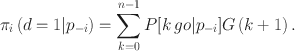
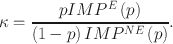
2.2 Impulse Balance Equilibrium: IBE
IBE basically assumes that if at some stage an alternative option would have yielded a higher payoff, then the agent receives an impulse to use this alternative in the next stage, i.e., agents only take account of foregone payoffs, as in Learning Direction Theory (Selten & Buchta, Reference Selten, Buchta, Budescu, Erev and Zwick1999). It is defined as the long run outcome of such stage-to-stage behaviour. In the context of market-entry games, an agent receives an impulse for entry if the payoff received from not entering is smaller than that from entering. Denoting by
 the number of other entrants and by
 the common probability of entering the market, the expected magnitude of these impulses for entry is defined as:
or equivalently in terms of
 rather than
 :
:
Similarly, an agent receives an impulse for no entry if the payoff received from entering is not larger than that from not entering. The expected magnitude of these impulses for no entry is defined as:
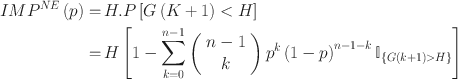
or equivalently

Note that these impulses are defined relatively to the game's maximin pure strategy of not entering the market which yields a sure payoff of
 . Selten and Chmura (Reference Selten and Chmura2008) further observe that receiving a payoff lower than this sure payoff should be perceived as a loss. To this extent, and in the light of empirical and experimental evidence of loss aversion in agents' preferences (Bernatzi & Thaler, Reference Bernatzi and Thaler1995; Tversky & Kahneman, Reference Tversky and Kahneman1991), we follow Ockenfels and Selten (Reference Ockenfels and Selten2005) and define an IBE for this market-entry game such that agent
 is indifferent between ‘receiving
 and entering’ and ‘receiving
 and not entering’, where
 stands for an impulse weight. That is, agent
 would choose to enter the market with probability
 that equalises her expected weighted impulses:

This impulse balance equation characterizes a long-run IBE in which participants do no more react to the expected impulses they receive. We could of course consider a short-run IBE, i.e., that would solve
 , but the resulting IBE for agent
 would then be independent of
 and, as shown in the next section, this would considerably limit the scope of our study.
Finally, unlike Selten and Chmura (Reference Selten and Chmura2008) who assume
 , we estimate the impulse weight
 by Maximum Likelihood (as for EvE) so the estimator of
 is
is
 and the MLE of
 (assuming symmetry and
 ) follows from
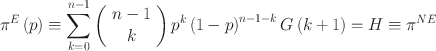
3 A specification test: the
 -test
-test

When we assume symmetry, the models we consider only propose a reparametrization
 for EvE and
 for IBE. Thus, under symmetry, there is no scope for discriminating between these models beyond commenting on implausible values of
 and
and
 . If we do not impose symmetry, then (3) and (7) can be rewritten as systems of linear restrictions on parameters
 and
and
 :
:

and

Both systems can thus be written in the form
 , with
 or
or
 , and with
 ,
,
 and
and
 vector functions with values in
 . The proposed formulation of (9) and (10) in terms of
 makes it possible to express the EvE or IBE model for homogenous players—in the sense that they share a common single parameter—while still allowing for possibly different individual entry probabilities, and to design a specification test. A further possibility we shall explore is to allow for cluster-heterogeneous players, i.e., players with similar characteristics (e.g., entry-probabilities) whom the model considers identical by assigning them the same parameter. In this case, θ is a vector instead of a scalar and the length of the vector directly affects the power of the
 -test since a vector of length
 represents full heterogeneity and leads to never rejecting the null of consistency.
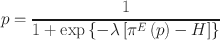
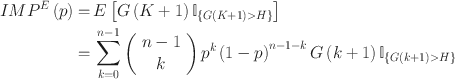
Given the asymptotically normal estimator
 of
of
 , the vector of individual entry frequencies, with asymptotic variance
 of which we describe a consistent estimator
 in Appendix III.A, an optimal asymptotic least squares estimator of
 isFootnote 8:

with
 converging to
 is thus the GLS estimator in the regression of
 on
on
 , the variance of the error term being
 .
.
Given a preliminary estimate of
 , say
, say
 obtained by replacing
 in (11) with the identity matrix, i.e.,
 is the OLS estimator in the regression of
 on
on
 , a consistent estimator of
 is:
is:
The asymptotic variance of
 is given by
 and a consistent estimator is
 . Under the null that there exists
 such that
 for the true
 , or in other words that the restrictions on entry probabilities embodied by the model are valid,

and this over-identification test can be used to test the underlying theory. All we need for the implementation of this specification test, for short the
 -test, are thus
 and the derivatives
 . The technical details for the determination of these expressions are given in Appendix III.B. The number of degrees of freedom is
 when assuming homogeneity [i.e., the length of vector
 is 1, cf. (12)] and it is at most
 when assuming heterogeneous players sorted in
 clusters (i.e., the length of vector
 is
is
 ), as discussed in Appendix III.C.
Note finally that since this test exploits the game’s probabilistic structure by rewriting agents’ probabilities of entry as a function of
 , it can be tailored for the assessment of behaviour in other binary-choice participation games like the volunteer’s game, the (discrete) step-level public good game and voter participation games. This, of course, remains conditional on having well-defined predictions to test, as is the case for EvE and QRE in general but not necessarily for IBE since its long-run equilibrium may not always be defined.Footnote 9
4 Experimental design and procedures
The experiments involve groups of 10 participants and a 2 × 3 factorial design which assumes two payoff levels, High and Low, and three payoff structures: one two-step payoff function (DISC) yielding a positive payoff
 from entering if attendance
 and 0 otherwise, and two non-monotone ones (NOM1 and NOM2) in which payoffs first increase and then decrease with
 . The binary payoff structure of DISC implies that the players’ choices are strict substitutes whereas the non-monotone structures introduce both strategic complementarity and strategic substitutability in the players’ actions that have been theoretically studied in the context of global congestion games (see e.g., Karp et al., Reference Karp, Lee and Mason2007) but which effects in complete information settings have not yet been investigated experimentally.Footnote 10
These payoff structures are displayed in Fig. 1, and the models’ equilibrium relationships between
 and
and
 or
or
 for the treatments considered are shown in Fig. 2. For each payoff level, both DISC and NOM1 yield
 Nash equilibria in pure strategies, unique mixed-equilibrium strategies and unique IBE strategies whereas NOM2 has one more equilibrium in pure strategies (where all agents choose not to enter), two mixed-equilibrium strategies and two IBE strategies (one with a low entry-probability and one with a high entry-probability).Footnote 11
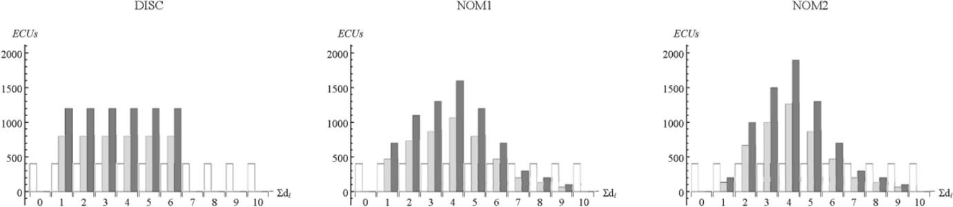
Fig. 1 Payoff levels and structures of market-entry games. No filling stands for ‘No Entry’, light gray (dark gray) stands for ‘Entry’ when payoffs are Low (High). Payoffs expressed in Experimental Currency Units—see Appendix IV.D for exact figures

Fig. 2 Relationship between
 and EvE’s
 or IBE’s
 . Thick (Thin) lines stand for High (Low) payoff levels. For EvE, the plots report the
 predictions for each payoff structure and level (cf. coloured horizontal lines). For IBE, the plots display the
 predictions (cf. dots) for each payoff structure and level. As
 ,
,
 in DISC and NOM1
We are interested in checking if and how behaviour is affected by these payoff structures and to what extent it is consistent with EvE and/or IBE when allowing for cluster-heterogeneity. In this regard, since the ranges of probabilities for which EvE and IBE yield model-consistent estimates in DISC and NOM1 are
 for EvE and
 for IBE, the models’ cluster-estimates should lie within these ranges and be significantly different from each other for cluster-heterogeneity to be model-consistent and significant. It thus follows that the scope for IBE to accommodate the latter in these treatments is considerably larger than that for EvE.Footnote 12
A similar argument holds for NOM2 since the mixed-equilibria have different loci of consistent choice frequencies (defined either on
 or on
or on
 with
with
 ) whereas the IBE equilibria have a unique locus (because both equilibria depend on a common
 ), so the identification of model-consistent clusters of participants playing in such different (Nash or IBE) equilibria can be achieved with IBE but not with EvE.
Our motivation to consider different payoff levels is to check whether the payoffs’ magnitude affects the presence of model-consistent clusters of players, and thus to possibly complement the findings of McKelvey et al. (Reference McKelvey, Palfrey and Weber2000) who report no significant payoff-magnitude effect on the participants’ QRE best-responsiveness in
 games and evidence of a heterogeneous play.
The experiments were conducted at the Laboratory for Experimental Economics of the University of Jaume I (Spain). Participants were undergraduate students in Business Administration, Law or Engineering and were recruited by public advertisement on campus. We conducted eight sessions per payoff structure (DISC, NOM1, NOM2) with 10 participants per session, totalling 240 individuals. For each payoff structure, we conducted four sessions with Low payoffs and four sessions with High payoffs. The experiments were conducted with a between-subject matching protocol and participants could play in only one session. Upon arriving in the laboratory, they were randomly assigned to cubicles equipped with computer terminals and were given instructions that were read aloud.Footnote 13 To avoid framing effects, we presented the game in neutral language by asking participants to choose between actions A and B. Each session involved 150 rounds of play, and at the end of each round, participants were only informed about the total number of players in their group who chose B ("No entry"), their own payoff in that round and their cumulated payoff. This information was appended to a "History" window that could be seen at any time during the experiment. Although participants played in fixed groups of 10, we believe that the provision of a sparse end-of-round information feedback combined with the relatively large number of players (10), and a relatively large ‘market size-to-capacity’ ratio (60%) renders entry-coordination very difficult to achieve. Each session lasted a maximum of 1 h, including the time needed to read the instructions. Participants were rewarded for each round of play at the rate of 0.02 € per 100 points and individual average earnings were €12.77 (i.e., €11.94 in the Low payoff sessions and €13.60 in High payoff ones).
5 Results
We start with an overview of the data by displaying the evolution of averaged entry probabilities and their polynomial fits in Fig. 3. The plots suggest an under-entry
 in all High payoff treatments, and that the ‘magic’
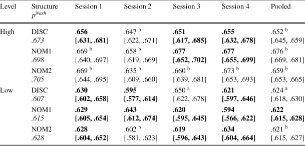
 is more likely to hold when payoffs are Low, especially in NOM1 and NOM2. These entry patterns are also present in the session data (cf. Appendix V) and in line with the session and treatment average entry rates of Table 1.

Fig. 3 Evolution of average probabilities of entry. Horizontal lines stand for the symmetric mixed-equilibrium predictions (we only consider the high-probability equilibrium of NOM2). Bold lines represent polynomial fits of degree 10
Table 1 Average entry probabilities
|
Level |
Structure
|
Session 1 |
Session 2 |
Session 3 |
Session 4 |
Pooled |
|---|---|---|---|---|---|---|
|
High |
DISC .673 |
. 656 [.631, .681] |
.647 b [.622, .671] |
.651 [.617, .685] |
.655 [.632, .678] |
.652 b [.645, .659] |
|
NOM1 .698 |
.669 b [.640, .697] |
.658 b [.619, .669] |
.677 [.652, .702] |
.677 [.655, .699] |
.676 b [.669, .681] |
|
|
NOM2 .705 |
.669 b [.644, .695] |
.635 b [.609, .660] |
.660 b [.639, .681] |
.673 b [.653, .693] |
.659 b [.653, .665] |
|
|
Low |
DISC .607 |
.630 [.602, .658] |
.595 [.577, .614] |
.650 a [.622, .678] |
.621 [.597, .646] |
.624 a [.618, .630] |
|
NOM1 .615 |
.629 [.605, .654] |
.643 [.612, .674] |
.620 [.595, .645] |
.594 [.566, .622] |
.622 [.615, .628] |
|
|
NOM2 .628 |
.628 [.604, .652] |
.602 b [.581, .623] |
.619 [.596, .643] |
.634 [.604, .664] |
.621 b [.615, .627] |

Each ‘session’ (‘pooled’) estimate refers to 1500 (6000) observations; Nash mixed-equilibrium predictions in italics; bold cells characterize instances where the symmetric mixed-equilibrium strategy cannot be rejected at the 5% level; 95% Confidence Intervals (based on Newey–West variance estimates) in brackets
aSignificant over-entry, i.e., when
 is smaller than the lower bound of the 95% CI
bSignificant under-entry, i.e., when
 is greater than the upper bound of the 95% CI
The treatment (pooled) figures of Table 1 show no support for the predicted ranking of entry rates
 . Pairwise comparisons indicate a substantially higher entry rate in NOM1 than in DISC and NOM2 when payoffs are High and similar entry rates when they are Low. They also significantly increase with the payoff level, as predicted in equilibrium and as reported by Zwick and Rapoport (Reference Zwick and Rapoport2002) who study the effect of ‘low’ and ‘high’ entry costs in treatments with a similar ‘market size-to-capacity’ ratio (50%). We summarise this overview of the pooled data as follows:
Observation 0: (A) There is under-entry when payoffs are High. When payoffs are Low, there is (1) over-entry in DISC, (2) a weak support for the Nash mixed-equilibrium play in NOM1, and (3) under-entry (with respect to the high probability equilibrium) in NOM2.
(B) The effect of the payoff structure is most salient when payoffs are High and yields a substantially higher average entry rate in NOM1. Average entry rates also significantly increase with the payoff level, as expected in equilibrium.
Before estimating the models, we briefly assess the symmetry of individuals’ entry probabilities. The bar-charts in Fig. 4 reveal minor differences in average entry probabilities between the sessions of a treatment, and large within-session disparities with clusters of participants displaying a similar entry behaviour.Footnote 14 The data also show no support for the ‘low probability’ mixed-equilibrium of NOM2 so we will always refer to the ‘high probability’ equilibrium of this treatment when discussing our estimation results.
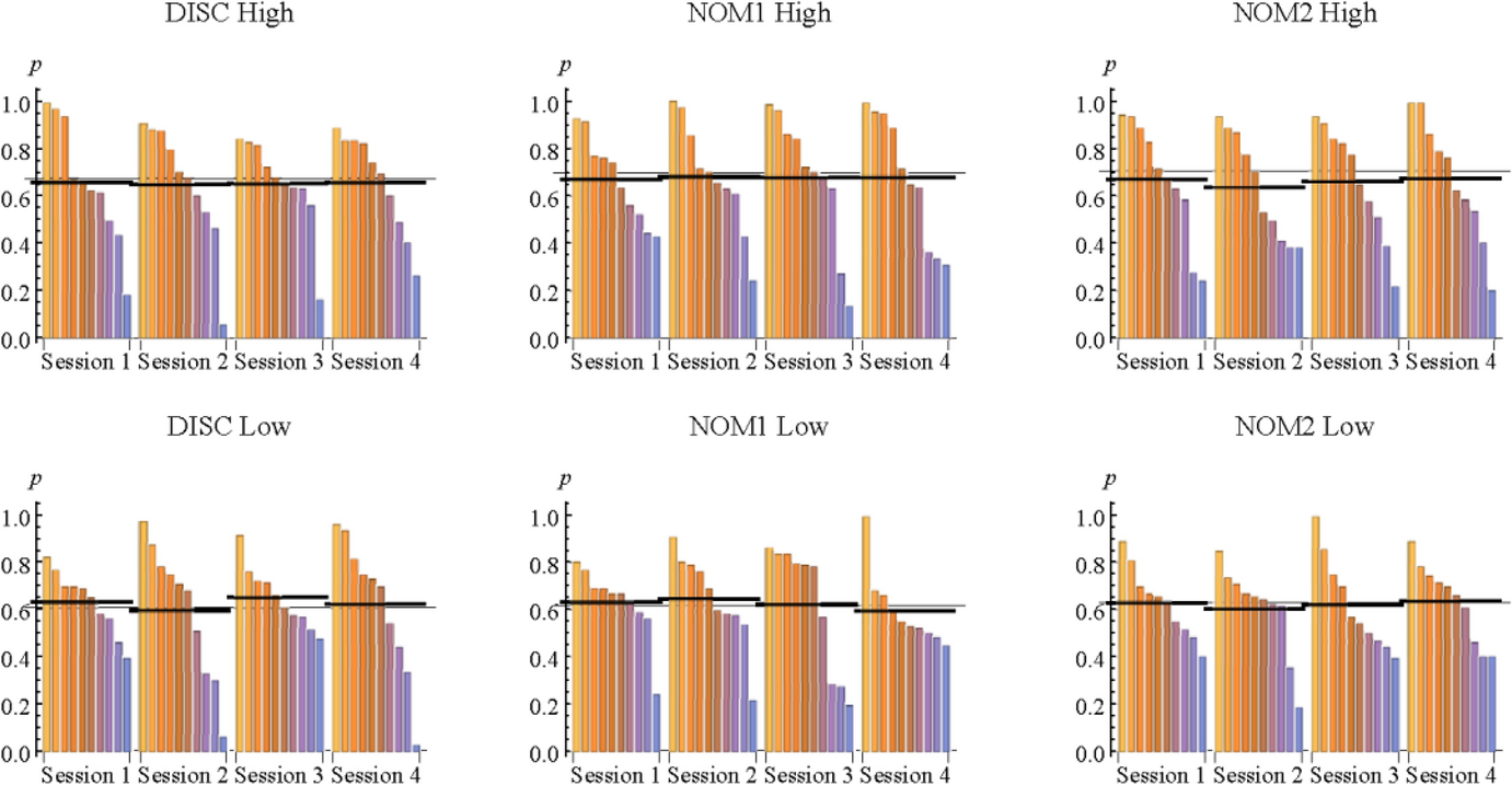
Fig. 4 Bar-charts of individual probabilities of entry. Each vertical bar represents an individual. Horizontal thin (thick) lines stand for the symmetric mixed-equilibrium predictions (average probabilities of entry)
5.1 Structural estimations when imposing symmetry
Table 2 reports the (pseudo-)Maximum Likelihood estimation outcomes of EvE and IBE when assuming symmetric players and unknown forms of autocorrelation and heteroskedascity in the errors. As the log-likelihood values contain no information about the model’s goodness-of-fit beyond the estimated probability of entry
 , we focus on the estimates’ overall consistency with Observation 0, and on their data-consistency, i.e., that a treatment’s session estimates are of similar magnitude and significance as the estimate for the pooled data.Footnote 15
Table 2 EvE and IBE estimates
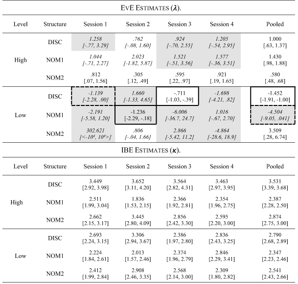
Each ‘session’ (‘pooled’) estimate refers to 1500 (6000) observations; 95% CIs based on Newey–West variance estimates in brackets; shaded cells characterize instances where the symmetric mixed-equilibrium strategy cannot be rejected at
 , cf. Table 1; (dashed-)framed cells characterize (almost) significantly negative estimates; italicised figures indicate insignificant estimates
 , i.e., maximal exploration in EvE.
Looking first at the outcomes for EvE, it appears that except for NOM2/High, all sessions report insignificant or inconsistent (negative) estimates no matter if
 is rejected or not (cf. shaded cells) or if their average entry rates indicate under-entry (cf. Table 1 and Fig. 4). Such insignificant estimates support maximal exploration whereas inconsistent ones result from EvE’s inability to rationalize over-entry when
 , as shown in Fig. 2. In the case of NOM2/High, they are all significantly positive and support a contained exploitation that is in line with the observed under-entry.
The pooled EvE-estimates indicate a contained exploitation in all High payoff structures and in NOM2/Low, and they are otherwise inconsistent (or almost so) as a result of over-entry. Thus, besides a significant under-entry in NOM2/High, the EvE-estimates provide no evidence of a data-consistent behaviour when the estimations impose a symmetric play.
This sharply contrasts with the outcomes for IBE since the session estimates are all significantly positive, typically larger when payoffs are High in DISC and NOM2, and similar across payoff levels in NOM1. This is confirmed by the treatments’ estimates which pairwise-comparisons further indicate that
 when payoffs are High and
 otherwise. We summarise the above in the following observation:
Observation 1: When assuming symmetric players and estimating the models with pseudo-Maximum Likelihood methods:
(A) The EvE-estimates are data-consistent in NOM2/High and indicate a contained exploitation that is in keeping with the observed under-entry. Otherwise, they are data-inconsistent: they mostly indicate maximal exploration whereas pooled estimates are either negative (thus inconsistent) or they support a contained exploitation.
(B) The IBE-estimates are data-consistent and in keeping with Observation 0. They indicate:
(1)
in DISC and NOM2, and
in NOM1.
(2)
when payoffs are High and
when they are Low.


5.2 Structural estimations when relaxing symmetry
We now estimate the models without imposing symmetry and we run our specification test to assess the consistency of estimates with the restrictions that either model imposes on individual behaviour. Note that the Σ-test only suits the analysis of session data, i.e., games with
 players.
For each session, we cluster the entry probabilities
 using the kmeans procedure (with 20 random initial values) and estimate each model and its inverse form with
 clusters; each cluster having its own
 -parameter (where
 is either to
 or
or
 ).Footnote 16 This generates eight specifications for each model and treatment which we estimate with OLS procedures. For each session, model (IBE and EVE) and value of
 , we select the ‘best’ specification in terms of the estimates’ theoretical consistency and the credibility of their confidence intervals. Next, for each session and model, we select the estimated specification with the smallest number of clusters,
 , needed to not reject the Σ-test at
 . Thus, the reported estimation results document the models’ non-rejections of the Σ-test when
 , and their rejections or non-rejections when
 . Noting that a rejection with
 can reasonably be seen as disqualifying the model when
 , we focus discussion on specifications that do not reject the Σ-test.
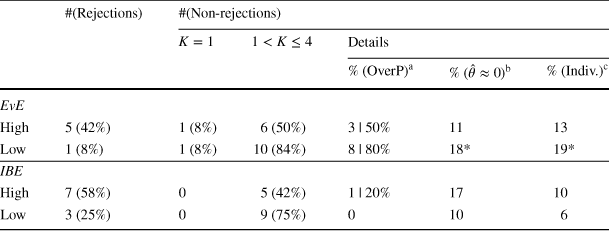
The estimation outcomes are relegated to Tables VII.A.1–4 in Appendix VII.A, and since they display no obvious pattern in terms of payoff structure, we start with summarising their main characteristics for each payoff level in the upper panel of Table 3. The first three columns tally the models’ rejections and non-rejections of the Σ-test when
 (i.e., homogeneity is not rejected) or when
 (i.e., homogeneity is rejected in favour of cluster-heterogeneity).
Table 3 Summary of specification test outcomes: OLS procedures

|
#(Rejections) |
#(Non-rejections) |
|||||
|---|---|---|---|---|---|---|
|
|
|
Details |
||||
|
%(OverP)a |
% (
|
% (Indiv.)c |
||||
|
All data |
||||||
|
EvE |
||||||
|
High |
3 (25%) |
3 (25%) |
6 (50%) |
6 | 100% |
45 |
37 |
|
Low |
1 (8%) |
5 (42%) |
6 (50%) |
2 | 33% |
52* |
38* |
|
IBE |
||||||
|
High |
7 (58%) |
0 |
5 (42%) |
1 | 20% |
22 |
12 |
|
Low |
3 (25%) |
0 |
9 (75%) |
1 | 11% |
10 |
6 |
|
Last 75 rounds |
||||||
|
EvE |
||||||
|
High |
0 |
6 (50%) |
6 (50%) |
6 | 100% |
55 |
43 |
|
Low |
0 |
6 (50%) |
6 (50%) |
5 | 83% |
56 |
54 |
|
IBE |
||||||
|
High |
4 (33%) |
0 |
8 (67%) |
4 | 50% |
27 |
18 |
|
Low |
2 (17%) |
0 |
10 (83%) |
5 | 50% |
27 |
17 |


There is a total of 12 sessions per payoff level;
 characterises homogenous players and
 cluster-heterogeneity; Detailed statistics refer to non-rejected specifications
a% of Over-Parametrised specifications with

b% of insignificant/inconsistent estimates
c% of individuals with insignificant estimates
*Including/relating to two inconsistent EvE estimates
EvE is not rejected for a total of 20 sessions (out of 24, 83%) whereas IBE is not rejected for a total of 14 sessions (58%). Of these non-rejected specifications, EvE supports cluster-heterogeneity in 12 sessions (60%) whereas all non-rejected IBE-specifications do so. The summary tables in Appendix VII further reveal that both models are rejected for 4 sessions and that both are not rejected for 14 others. Since the remaining 6 sessions (25%) reject only IBE, it appears that EvE organises best the observed behaviour.
We proceed with checking whether the cluster-estimates of a specification (session) are heterogeneous with pairwise
 -tests of equality and note that when all pairwise-tests are rejected, the estimates are considered heterogeneous if all pairwise-tests are also rejected when assuming
 clusters and the clusters were nested – the pairwise test outcomes are summarised in the last columns of Tables VII.A.1–4 in Appendix VII.A. On the other hand, a single non-rejection of equality implies that the specification is over-parametrised so the estimated cluster parameters are unreliable and one can only conclude that it has at most
 clusters.
The last three columns of Table 3 refer to the non-rejected specifications of a treatment and report the percentages of (1) over-parametrised multi-clustered specifications, (2) insignificant or inconsistent estimates and (3) individuals affected by such estimates. The models sharply differ according to these criteria as EvE’s specifications are far more likely to be over-parametrised than the IBE ones no matter the payoff level, i.e., a five-fold (three-fold) percentage difference when payoffs are High (Low). Most estimates of non-over-parametrised EvE-specifications are insignificant and none of these specifications yields estimates that fulfil the conditions to be considered heterogeneous. As for IBE, all estimates of non-over-parametrised specifications comply with these conditions when
 which leads us to conclude that, as expected, IBE accommodates cluster-heterogeneity better that EVE (cf. Sect. 4). Finally, about 50% of EvE’s estimates are insignificant and affect some 37% of individuals no matter the payoff level whereas for IBE the figures drop at least by half, especially when payoffs are Low.
We highlight treatment differences by assigning to each participant the
 -estimate of the cluster s/he belongs to and by comparing the resulting cumulative distributions of estimates for High and Low payoffs in each payoff structure. These distributions are displayed in Fig. 5 (with the samples’ median estimates)—insignificant estimates were set equal to 0. To document the effect of the
 -test on inference, the plots assume either (1) all estimates regardless of the sessions’
 -test outcomes (cf. dashed lines), or (2) estimates of non-rejected specifications only (cf. plain lines). In this regard, the distributions pertaining to (1) and (2) reveal important differences only when non-rejected specifications are seldom, as for IBE in NOM2/High.

Fig. 5 Cumulative distributions of individuals’ OLS estimates. Thick (Thin) lines stand for High (Low) payoff levels—dashed lines refer to the
 estimates of a treatment regardless of the
 -test outcomes. Insignificant estimates are set equal to 0. The plots report the estimates medians and numbers of non-rejected specifications (in brackets). The CDFs assume a maximum
 - and
- and
 -estimates of 5 and 15, respectively
The distributions’ large steps witness the presence of prominent clusters. In the case of EvE, the most prominent clusters consist of insignificant estimates and are found in DISC and NOM1 no matter the payoff level. There are also noticeable clusters of relatively large estimates supporting a more intense exploitation when payoffs are Low in DISC (with
 for over 20% of participants) and in NOM2 (with
 for about 40%). Such larger estimates counter-intuitively suggest that for these participants, exploitation is more intense when payoffs are Low. This contrasts with NOM1 where the distributions are more alike across payoff levels and support the prediction that exploitation intensifies with payoffs, as the median estimates also qualitatively suggest.
As for IBE, the distributions look similar in NOM1 and suggest no particular ‘payoff magnitude’ effect. They also display no prominent clusters of large estimates and thus contrast with the distributions of DISC and NOM2 which both do when payoffs are High (
 for about 30% of participants in these treatments). The presence of such clusters in those treatments identifies participants with low entry-rates, and their absence in NOM1 is in line with Observation 1(B): (1) the distributions and median estimates suggest that
 in DISC and NOM2, and
 in NOM1, and (2) the median estimates support
 when payoffs are High.
We attribute the absence of such clusters in NOM1 and the higher participation in NOM1/High to the relatively lower risk of regretting to enter that this structure entails when compared to DISC (which yields zero payoffs in case of over-entry) or to NOM2 (which bears an incentive to enter to avoid the risk of under-entry but which highest payoffs obtain only when
 , cf. Appendix IV.D).
All in all, allowing for cluster-heterogeneity in the estimations reveals important differences in the models’ explanatory powers and indicates that IBE outperforms EvE in this regard. We summarize this as follows:
Observation 2: When relaxing symmetry and estimating the models with OLS procedures, the null of the
 -test is less likely to be rejected by EvE than by IBE (17% vs 42% of all sessions, respectively). However, when compared to IBE, the non-rejected EvE-specifications are: (1) less likely to reject homogeneity, (2) more likely to be over-parametrised, (3) more likely to generate insignificant or inconsistent estimates that affect a larger proportion of participants, and (4) unable to rationalise the presence of clusters of players with low entry-probabilities. Thus IBE accommodates cluster-heterogeneity better than EvE.
We conduct the same analysis for the last 75 rounds to check for a possible experience effect in the observed behaviour. The tests’ outcomes are summarised in the lower panel of Table 3—see Tables VII.B.1–4 in Appendix VII.B for detailed results.Footnote 17 Now EvE is not rejected for all sessions whereas IBE is not rejected for 18 of them (75%, instead of 58% when accounting for all rounds) mostly with Low payoffs. Homogeneity (
 ) is again rejected for IBE in all sessions, and it is not for EvE in 12 sessions so that 50% of EvE-specifications are multi-clustered (instead of 60%). These specifications also display fewer clusters only when assuming EvE in DISC and NOM1/High so behaviour in these treatments would become more homogenous in the long run according to EvE. Overall, since both models are not rejected for 18 (75%) sessions and the remaining 6 reject IBE but not EvE (cf. Appendix VII.B), EvE would appear again to organise the observed behaviour best.
Looking into the specifications’ details, we find that the models yield more non-rejected over-parametrised specifications: over 83% for EvE, and 50% for IBE no matter the payoff level. There is also no evidence of heterogeneous estimates in the unique non-over-fitted EvE-specification (cf. NOM1/Low/Session 1) whereas all IBE-specifications with
 are heterogeneous. The models’ differences remain in terms of insignificant estimates, with 55% of EvE-estimates indicating maximal exploration and affecting about 50% of participants whilst only 27% of the IBE ones are insignificant and concern 17% of participants no matter the payoff level.
The distributions of estimates in Fig. 6 tend to confirm the patterns found when assuming all data and they are moderately affected by the data-attrition resulting from the
 -test rejections. Insignificant EvE-estimates are frequent in all treatments but NOM2/Low, where the estimates support a contained exploitation and the null of homogeneity (
 ) in all sessions. Otherwise, the distributions pertaining to DISC and NOM2 still counter-intuitively suggest that it increases when payoffs are Low whereas those of NOM1 comply with the alternative that exploitation increases with payoff levels.
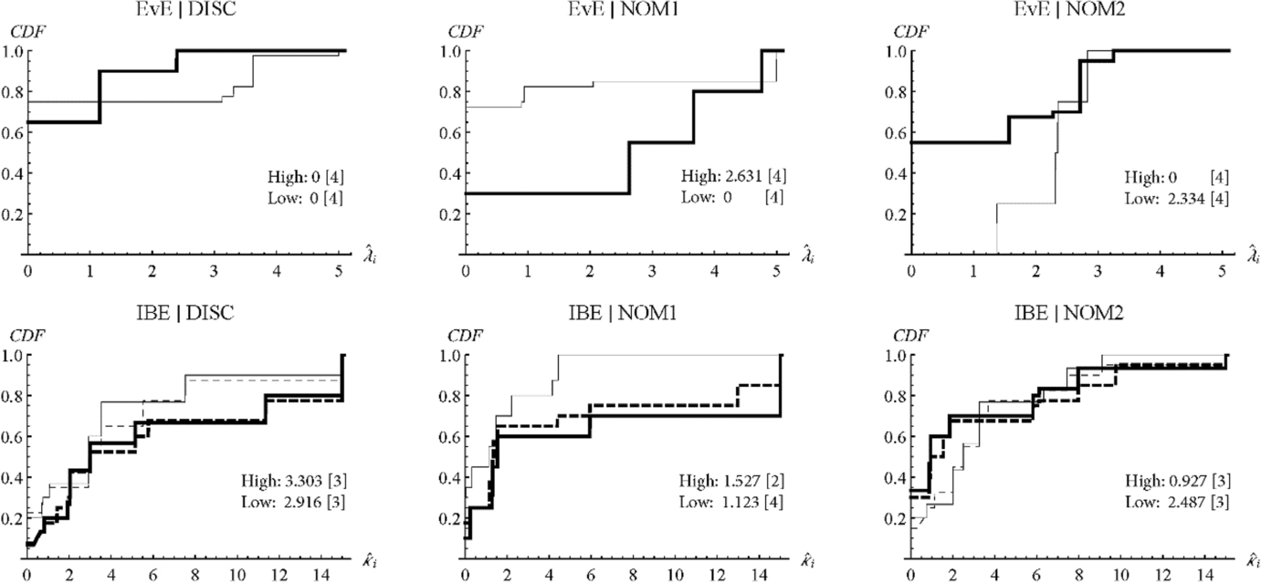
Fig. 6 Cumulative distributions of individuals’ OLS estimates (last 75 rounds). Thick (Thin) lines stand for High (Low) payoff levels—dashed lines refer to the
 estimates of a treatment regardless of the
 -test outcomes. Insignificant estimates (at
 ) are set equal to 0. The plots report the estimates medians and numbers of non-rejected specifications (in brackets). The CDFs assume a maximum
 - and
- and
 -estimates of 5 and 15, respectively
For IBE, the distributions and median estimates of DISC look alike those in Fig. 5 whilst those of NOM1 and NOM2 reveal (1) a drop in the median estimate of NOM1/Low and the presence of a cluster with large
 -estimates in NOM1/High, and (2) the absence of such a cluster in NOM2/High. However, the evolution of play in session data suggests that such higher (lower) participation for some participants in NOM1/Low and NOM2/High (NOM1/Low) are actually due to an ‘end-game effect’ in the last 10–20 rounds of these treatments, cf. Appendix V. This leads to the following observation:
Observation 3: When relaxing symmetry and estimating the models with OLS procedures and the data of the last 75 rounds:
(A) The null of the
 -test is less likely to be rejected by EvE than by IBE (0% of all sessions vs 25% for IBE).
(B) Non-rejected EvE-specifications in DISC/High and especially NOM1/High have fewer clusters so behaviour becomes more homogenous in the long run according to EvE.
(C) The features 1) to 4) of EvE’s non-rejected specifications outlined in Observation 2 hold and confirm IBE’s superior ability in organising the observed behaviour.
We proceed with a second robustness check of Observation 2 by estimating the models with more efficient procedures that possibly call for (‘naïve’ or Tikhonov) regularisation of the error variance matrix to address the unstable results we got when estimating the models with GLS methods. We thus consider five minimum-distance estimators in addition to the OLS and GLS ones, and we allow for regularisation whenever it is deemed necessary to give the models their best shot at organising the data.Footnote 18 That is, we estimated the models and their inverse forms for each session with seven estimators and with
 clusters, generating over 80 specifications per model and treatment. For each model and value of
 , we selected the specification that best addresses a set of criteria regarding the theoretical consistency of parameter estimates and the credibility of their confidence intervals, but also to the condition number of the variance matrix of the error terms (not too large) and to the magnitude of the efficiency gains relative to OLS (not too large but not negligible).
The selected
 -specifications are reported in Tables I to IV of Appendix VII.C and indicate that some form of regularisation is needed for 19 sessions (79%) when estimating EvE and for only 2 (8%) when estimating IBE.Footnote 19 The
 -test outcomes and the main characteristics of the models’ non-rejected specifications are summarised in Table 4. They first indicate that the use of regularisation marginally affects the
 -test outcomes for EvE and leaves those for IBE idle. Also, both models are not rejected for 13 sessions (instead of 14 when using OLS methods), EvE is not rejected for 6 (25%) and IBE for only 1 session (instead of 0).
Table 4 Summary of specification test outcomes with(out) regularisation
|
#(Rejections) |
#(Non-rejections) |
|||||
|---|---|---|---|---|---|---|
|
|
|
Details |
||||
|
% (OverP)a |
% (
|
% (Indiv.)c |
||||
|
EvE |
||||||
|
High |
5 (42%) |
1 (8%) |
6 (50%) |
3 | 50% |
11 |
13 |
|
Low |
1 (8%) |
1 (8%) |
10 (84%) |
8 | 80% |
18* |
19* |
|
IBE |
||||||
|
High |
7 (58%) |
0 |
5 (42%) |
1 | 20% |
17 |
10 |
|
Low |
3 (25%) |
0 |
9 (75%) |
0 |
10 |
6 |


There is a total of 12 sessions per payoff level;
 characterises homogenous players and
 cluster-heterogeneity; Detailed statistics refer to non-rejected specifications
a% of over-parametrised specifications with

b% of insignificant/inconsistent estimates
c% of individuals with insignificant estimates
*Including/relating to two inconsistent EvE estimates
The effect of regularisation is more salient on the estimates since the models become comparable in terms of rejecting homogeneity (i.e., 22 sessions for EvE vs 24 sessions for IBE), the proportion of insignificant/inconsistent estimates and, to a lesser extent, the proportion of individuals with such estimates. Yet, over 50% of EvE’s non-rejected specifications are still over-parametrised whereas less than 20% of the IBE-ones are so.
The plots in Fig. 7 refer to heterogeneous samples of estimators and appear again to be affected by the
 -test results only when the available data is sparse, as for EvE in NOM2/High. Insignificant EvE-estimates are mostly found in DISC/Low and NOM2/High, and they are about equally frequent no matter the payoff level in NOM1. Otherwise, the distributions of IBE-estimates, like those of EVE-estimates in DISC, display similar patterns as those referring to OLS estimates, cf. Fig. 5. The most noticeable changes occur for the EVE-estimates of NOM1 and NOM2: they are now most similar across payoff levels in NOM1 and suggest no particular payoff magnitude effect (like the IBE-distributions of this treatment) whereas they are mostly different in NOM2, with stochastically larger (and mostly homogenous) cluster-estimates when payoffs are Low.
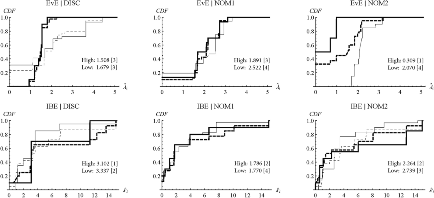
Fig. 7 Cumulative distributions of individuals’ (regularized) estimates. Thick (Thin) lines stand for High (Low) payoff levels—dashed lines refer to the
 estimates of a treatment regardless of the
 -test outcomes. Insignificant estimates are set equal to 0. The plots report the estimates medians and numbers of non-rejected specifications (in brackets). The CDFs assume a maximum
 - and
- and
 -estimates of 5 and 15, respectively
Overall, this robustness analysis confirms the models’ respective (in)sensitivity to the symmetric assumption (Observation 1) and IBE’s superior ability to diagnose a model-consistent cluster-heterogeneity in the observed behaviour (Observation 2). We summarise the above in the following final observation:
Observation 4: When relaxing symmetry and using (naïve or Tikhonov) regularisation procedures when estimating the models with GLS or distance-based estimators (instead of OLS estimators):
(A) EvE is still less likely to reject the null of the
 -test (25% of all sessions vs 42% for IBE).
(B) The features 1) to 4) of EvE’s non-rejected specifications outlined in Observation 2 hold and confirm IBE’s superior ability in organising the observed behaviour.
(C) Our conclusions for IBE are hardly affected by the use of regularisation procedures.
6 Conclusion
In this paper we propose a novel approach to the analysis of symmetric participation games that checks the consistency of a model’s estimates with the restrictions it imposes on individual behaviour. This approach relaxes the model’s assumption of symmetry by allowing for the existence of clusters of players with similar observable characteristics, and it assesses how much cluster-heterogeneity a model can tolerate to still be consistent with its behavioural restrictions by means of a specification test. Thus, besides offering an alternative to the usual assessment of a model in terms of its goodness-of-fit, this approach allows for individual differences to be accounted for in a model-consistent way and therefore contributes to the literature on modelling heterogeneity in static games, see e.g., Rogers et al. (Reference Rogers, Palfrey and Camerer2009) and Golman (Reference Golman2011).Footnote 20
We assessed this approach with data on market-entry experiments which we analyse in terms of two stationary models: Exploitation versus Exploration (EvE, which is equivalent Logit-QRE) and Impulse Balance Equilibrium (IBE). Our empirical analysis sheds new light on the models’ sensitivities to the assumption of symmetric players or of cluster-heterogeneity and to the econometric procedures used. We summarise our findings in the following four points.
First, estimating EvE with the usual assumption of symmetric and homogenous players provides limited insight into the analysis of behaviour in these games because (1) the session estimates are largely invariant to treatment conditions and mostly support a maximal exploration (or purely random behaviour), and (2) the estimates for the pooled data are seldom consistent with session estimates. In this regard, IBE outperforms EvE.
Second, when allowing for cluster-heterogeneity and estimating the models with OLS methods, the null of the specification test is less likely to be rejected for EvE, and EvE is more likely to support homogeneity than IBE. However, the estimated specifications have considerably more insignificant cluster-estimates and are typically over-parametrised, so IBE also outperforms EvE in terms of accommodating cluster-heterogeneity. This holds when the estimations pertain to the second half of the experiments to account for participants’ experience of play.
Third, our approach can unveil behavioural patterns such as the presence of clusters of players with low-entry rates in some treatments and may explain them, i.e., such clusters are absent in treatments where payoffs remain positive when participation is over-capacity (as in NOM1) and they are present in treatments where the risk of experiencing a regret from entering is more salient (as in DISC and NOM2).
Fourth, when estimating the models with more efficient procedures (i.e., GLS or distance-based estimators that possibly allow for regularisation) our conclusions for IBE are hardly affected whereas those for EvE change considerably: homogeneity is then always rejected (like for IBE when assuming OLS methods) and insignificant or inconsistent cluster-estimates are less frequent. Yet, IBE still accommodates cluster-heterogeneity better than EvE.
Finally, the proposed approach is flexible enough to also allow an assessment of which type of heterogeneity is most consistent with some behavioural model, e.g., gender, socio-demographics, or any relevant mixture of observable characteristics. For example, it can be used to reveal a gender and/or a socio-demographic effect in the players’ participation, and the specification test could determine whether this effect (or which of these effects) is consistent with the symmetric model considered.Footnote 21 It can also be applied to test predictions regarding the sorting of players into clusters of individuals who either always or never participate as a result of reinforcement learning, as Duffy and Hopkins (Reference Duffy and Hopkins2005) predict and find. This, however, would raise the more challenging question of the formation of such clusters over time and its consistency with the type of learning considered. In this regard, our approach provides some first insights which we hope will be further explored.
Acknowledgements
We thank Jacob Goeree, Ted Turocy, Tom Wilkening, and audiences at Aix-Marseille School of Economics (GREQAM), University of Melbourne, University of New South Wales, Queensland University of Technology, the International Meeting of the Economic Science Association (Hawaii), the Australia New-Zealand Workshop in Experimental Economics (Melbourne), the Workshop on Behavioral and Experimental Economics (Aix-en-Provence), the 11th Workshop on Complexity: Theory and Experimental Analyses (Nice), and the École des Hautes Études en Sciences Sociales (CAMS, Paris) for useful comments, as well as, in retrospect Reinhard Selten who suggested that we look into the Impulse Balance Equilibrium of this game. We also thank Nikolaos Georgantzis who generously gave us access to the Laboratory for Experimental Economics at Universidad Jaume I (Castéllon, Spain) to run the experiments, Raquel Barreda and Juan Gómez for their assistance in their conduct, and Yohan Mathis and Mathilde Saguin for able research assistance on parts of the statistical analysis at the University of Strasbourg. We are grateful to the Editor, John Duffy, and two anonymous reviewers for valuable comments that greatly improved the presentation of our findings. Support from the European Commission through the Laboratoires Européens Associés, the Institute for Economic Analysis (Barcelona) and the University of Côte d’Azur (Nice, Project UCAinACTION of ANR-15-IDEX-01) where parts of this research were conducted, and the Australian Research Council (DP140102949) is gratefully acknowledged. The usual disclaimer applies.
Funding
Open Access funding enabled and organized by CAUL and its Member Institutions.


 p
p λ
λ κ
κ pNash
pNash pNash
pNash κ→∞
κ→∞ p→0
p→0


 4×10
4×10 Σ
Σ λ^i
λ^i κ^i
κ^i
 4×10
4×10 Σ
Σ α=5%
α=5% λ^i
λ^i κ^i
κ^i

 4×10
4×10 Σ
Σ λ^i
λ^i κ^i
κ^i


 Open access