1 Introduction

Expected Utility Theory (EUT) is one of the oldest and widely used criteria for decision making under risk. Bernoulli (Reference Bernoulli1738) first proposed EUT to resolve the St. Petersburg Paradox. Von Neumann and Morgenstern (Reference von Neumann and Morgenstern1947) provided a normatively appealing axiomatization of EUT. Yet, Allais (Reference Allais1953) challenged the descriptive accuracy of EUT with two examples. His first example (Allais, Reference Allais1953, p. 527) is known as the Allais Paradox or common-consequence effect. Following MacCrimmon and Larsson (Reference MacCrimmon, Larsson, Allais and Hagen1979), his second example (Allais, Reference Allais1953, p. 529) is known as the common-ratio effect. One illustration of this effect, due to Kahneman and Tversky (Reference Kahneman and Tversky1979, p. 266), is that subjects choose $3,000 for sure over an 80% chance of winning $4,000 but choose a 20% chance of $4,000 over a 25% chance of $3,000 (when probabilities are scaled down by the same ratio, which gives the effect its name).

A wide-spread perception is that the common-ratio effect is a robust behavioral regularity. More than 40 years ago MacCrimmon and Larsson (Reference MacCrimmon, Larsson, Allais and Hagen1979, Sect. 5.3, p. 369) concluded that “even though the common-consequence problem … is generally called the ‘Allais Paradox’, the [common-ratio effect] which is also due to Allais is more of a ‘paradox’ (if either is) in the sense that it elicits a higher rate of violation of the [EUT] axioms.” Given that the effect has since been tested in numerous studies, we can verify its experimental robustness. Our methodology is similar in spirit to meta-studies: we re-analyze experimental data collected in previous studies (meta-studies re-analyze previously published statistics).

Blavatskyy et al. (Reference Blavatskyy, Ortmann and Panchenko2022) re-analyzed data from 29 articles (81 experimental designs/ parameterizations, 8,947 observations) on the Allais Paradox and found that the standard paradox was recorded in 38 designs (46.9%), no paradox was recorded in 27 designs (33.3%) and the reverse paradox was recorded in the remaining 16 designs (19.8%). Here we reexamine data from 39 articles with 143 experimental parameterizations of the common-ratio effect (14,909 observations). Out of these 143 designs, the standard common-ratio effect was found in 85 designs (59.4%), no common- ratio effect was found in 43 designs (30.1%), and the reverse common-ratio effect was found in the remaining 15 designs (10.5%).

Our econometric analysis shows that the common-ratio effect is susceptible to similar effects of experimental design, implementation, and parameter choices as the Allais Paradox. Specific choices of an experimenter can make the common-ratio effect appear, disappear, or reverse. It is important to raise awareness of such effects to promote the development of appropriate non-expected utility theories that can rationalize these effects.

The remainder of the paper is organized as follows. In Sect. 2, we briefly explain the common-ratio effect. In Sect. 3, we explain how we collected the data. In Sect. 4, we provide our regression analysis. In Sect. 5, we offer a concluding discussion.

2 The common-ratio effect

The original Allais (Reference Allais1953, p. 529) example of the common-ratio effect is the following: A decision maker can prefer ₣100 million for certain over 98% chance of ₣500 million (and a 2% chance of nothing) and, at the same time, she can prefer 0.98% chance of ₣500 million (and a 99.02% chance of nothing) over a 1% chance of ₣100 million (and 99% chance of nothing). In the second binary choice problem, the chances of positive gains are scaled down from the corresponding chances in the first binary choice problem by a common ratio of 1/100. This gives the effect its name.

The common-ratio effect is illustrated in the probability triangle (Machina, Reference Machina1982) in Fig. 1 (axes not to scale). Point A (0,0) represents the prospect of ₣100 million for certain. Point B (0.02, 0.98) represents a 98% chance of ₣500 million. Point C (0.99,0) represents a 1% chance of ₣100 million. Point D (0.9902, 0.0098) represents a 0.98% chance of ₣500 million. Due to the scaling by a common ratio, line AB is parallel to line CD. The left panel of Fig. 1 shows a typical family of indifference curves for an expected-utility maximizer—positively-sloped parallel straight lines. Since AB is parallel to CD, A is located on a higher indifference curve than B (as shown on the left panel of Fig. 1) if and only if C is located on a higher indifference curve than D. Thus, an expected-utility maximizer weakly prefers A over B if and only if she weakly prefers C over D (a risk-averse choice pattern consistent with EUT).

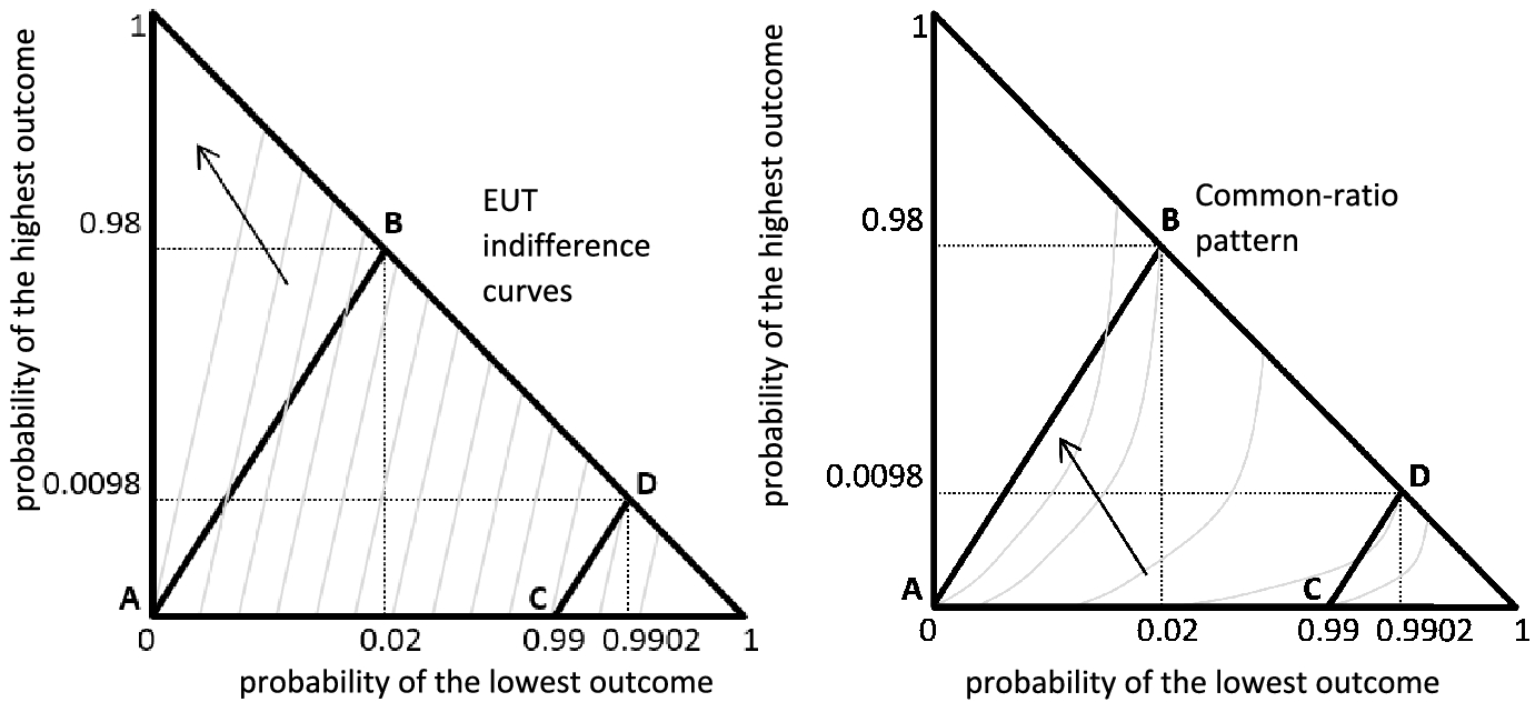
Fig. 1 Illustration of the common-ratio effect in the probability triangle (not to scale)

A choice of A over B and D over C violates EUT (except for a special case of indifference) and we refer to this choice pattern as the common-ratio pattern. The right panel of Fig. 1 illustrates the common-ratio choice pattern. A decision maker who chooses B over A and C over D likewise violates EUT and we call this the reverse common-ratio pattern. Typically, the majority of decision makers reveal the common-ratio choice pattern and only a minority reveal the reverse common-ratio pattern. It is these behavioural regularities that became known as the common-ratio effect.

Several design, implementation, and parameter choices could affect the likelihood of observing the common-ratio effect. First, a small common ratio reduces the difference in expected utility between lotteries in the second binary choice (“scaled-down” lotteries C and D). Loomes (Reference Loomes2005, p. 305) argued that this may increase certain instances of the common-ratio effect when decision makers are prone to Fechner (Reference Fechner1860/1966)-type random errors. Such errors are more likely in the second binary choice between “scaled-down” lotteries C and D, which differ little in expected utility, compared to the first binary choice between “scaled-up” lotteries A and B, which differ considerably in expected utility.

Second, the slope of lines AB and CD in the probability triangle might influence the likelihood of the common-ratio effect. Note that the slope of lines AB and CD in the probability triangle is an increasing function of the probability of the highest outcome in risky lottery B in the first common-ratio question. Loomes and Sugden (Reference Loomes and Sugden1998) experimented with several different slopes and found that parameterizations with higher slopes generally reveal higher instances of the common-ratio effect. Parameterizations with higher slopes create a similarity (or inconsequentiality) of probabilities in the second common-ratio problem (the probability of a non-zero outcome in lottery D becomes relatively similar to that in lottery C). This similarity (or inconsequentiality) can catalyze the common-ratio effect. Blavatskyy et al. (2020) reanalyzed experimental data from 81 experiments reported in 29 studies of the Allais Paradox and found that a relatively low slope in the probability triangle is likely to reverse the Allais Paradox. We test if this conclusion also holds for the common-ratio effect.

Third, instances of the common-ratio effect may be affected by the sheer size of monetary outcomes. Lotteries with larger outcomes may induce more risk-averse choices. Ceteris paribus, this increases the likelihood of EUT-consistent risk-averse choice pattern A≿B and C≿D.

Fourth, Blavatskyy (Reference Blavatskyy2010, experiment 2, pp. 232–5) found that the common-ratio effect not only disappears but is reversed when the medium outcome is moved away from the highest outcome. A parameterization with a relatively high ratio of middle to highest outcome may increase cognitive load making both common-ratio questions a harder decision problem, which might lead to a higher rate of EUT violations. Blavatskyy et al. (2020) found that the Allais Paradox is more likely in experiments with the medium outcome being close to the highest outcome.

Fifth, instances of the common-ratio effect may be affected by the nature of the incentives used in experimental studies. Debate is ongoing about the effects of hypothetical and real incentives in experimental economics. On the one hand, Kahneman and Tversky (Reference Kahneman and Tversky1979, p. 265) argued in favor of hypothetical incentives in experiments on individual choice under risk. On the other hand, financial incentives are the default choice in most economics experiments and there are good reasons for it (e.g., Hertwig & Ortmann, Reference Hertwig and Ortmann2001; Ortmann, Reference Ortmann, Svorencik and Maas2016). Hertwig and Ortmann (Reference Hertwig and Ortmann2001) argue that the choice of hypothetical or real incentives ought to be evidence-based.

Sixth, Carlin (Reference Carlin1992) found that the common-ratio effect is less likely when choice alternatives are represented as compound lotteries or in a frequency format rather than as simple probability distributions. In their meta-study, Blavatskyy et al. (2020) found such an effect for the Allais Paradox. To summarize, we identify six design and implementation details and parameter choices that might drive the results of experimental studies on the common-ratio effect: 1) common ratio itself; 2) slope of lines AB and CD in the probability triangle; 3) size of payoffs; 4) ratio of the middle to the highest outcome; 5) whether incentives are hypothetical or real; and 6) presentation of choice alternatives.

3 Data

We searched in the Scopus database with a string ( TITLE-ABS-KEY ( "common ratio") AND TITLE-ABS-KEY ( "experiment")) excluding non-economic articles, theoretical articles, and experimental studies that collect no data on the common-ratio effect (e.g., Andreoni & Sprenger, Reference Andreoni and Sprenger2012; Kelsey & Schepanski, Reference Kelsey and Schepanski1991; Müller-Trede et al., Reference Müller-Trede, Sher and McKenzie2018). To this list, we added articles identified in the process of data collection for our previous study (Blavatskyy et al. 2020) when in effect the authors collected experimental data on the common-ratio effect (some papers refer to the common-ratio problem as the Allais paradox, e.g., van de Kuilen & Wakker, Reference van de Kuilen and Wakker2006; Herrmann et al., Reference Herrmann, Hübler, Menkhoff and Schmidt2017). We discarded several experimental studies with unconventional parameterizationsFootnote ¹ as well as between-subject testsFootnote ² of the common ratio. Raw experimental data of Kahneman and Tversky (Reference Kahneman and Tversky1979) are lost and we cannot infer the frequencies of four choice patterns revealed in their common-ratio experiment. Starmer and Sugden (Reference Starmer and Sugden1989b) use the same experimental data as Starmer and Sugden (Reference Starmer and Sugden1989a). Birnbaum et al. (Reference Birnbaum, Schmidt and Schneider2017) re-analyze data of Birnbaum and Schmidt (Reference Birnbaum and Schmidt2015). This results in a list of 24 articles. Going through the references in these articles we identified another eight studies that collect data on the common-ratio effect. After circulating the first draft of our working paper we received feedback about seven additional recent studies collecting data on the common-ratio effect. With this final addition, we obtained 39 articles (preceded by an asterisk in the list of references). Data collected from these 39 articles (143 design/parameterizations with 14,909 revealed-choice patterns) are presented in Table 1.

Table 1 Experimental data on the common-ratio effect

In the first column of Table 1 we list the different experimental designs/parameterizations. In column 2 we enumerate the number of corresponding participants. Columns 3–6 of Table 1 list how many subjects revealed the four possible choice patterns (risk-averse and risk-seeking EUT-consistent choice patterns, common-ratio and reverse common-ratio choice patterns). Conlisk (Reference Conlisk1989) developed a test statistic, known as Conlisk z-statistic, which takes values close to zero under the null-hypothesis of there being no EUT violations. Large positive values of the statistic indicate that common-ratio choice patterns outnumber reverse common-ratio choice patterns. Large negative values of the statistic indicate the opposite (reverse common-ratio choice patterns outnumber common-ratio choice patterns). Columns 7 and 8 of Table 1 list Conlisk z-statistic and its corresponding p-value for each of 143 design/parameterizations.

The remaining columns of Table 1 show the realizations of the six design and implementation characteristics identified in the previous section as potentially relevant for instances of the common-ratio effect. Column 9 lists the probability of the highest outcome in risky lottery (B) in the first question (which is an increasing function of the slope of lines AB and CD in the probability triangle). Column 10 lists the common-ratio factor. Column 11 lists the highest outcome and its currency. Column 12 lists the ratio of middle to highest outcome. Column 13 is a dummy variable that equals one (zero) if the researchers used real (hypothetical) incentives. Column 14 shows whether choice alternatives were presented as simple lotteries (1), in frequency form (0*), or as compound lotteries (0). The last column is a dummy variable equal to one if experimental subjects were students.

The sources from which we collected data reported in Table 1 are listed in Table 2 (for 39 experimental articles). We do not consider data from stages 2 and 3 in the experiment of Baillon et al. (Reference Baillon, Bleichrodt, Liu and Wakker2016), repetitions 2–4 in Birnbaum and Schmidt (Reference Birnbaum and Schmidt2015), stages 2 and 3 in the experiment of Bone et al. (Reference Bone, Hey and Suckling1999), repetition 2 in Loomes and Sugden (Reference Loomes and Sugden1998) and repetitions 2–3 in Schmidt and Neugebauer (Reference Schmidt and Neugebauer2007) to avoid any confounding with the learning effects. We do not consider household-decision making in Bateman and Munro (Reference Bateman and Munro2005) to focus only on individual choice. We do not consider the repeated-play condition in Barron and Erev (Reference Barron and Erev2003) or the 10-play and 100-play conditions in DeKay et al. (Reference DeKay, Schley, Miller, Erford, Sun, Karim and Lanyon2016) to focus only on single realization of lotteries. Buschena and Zilberman (Reference Buschena and Zilberman1999, p. 261) report that 39% of subjects reveal common-ratio choice pattern in questions 1 and 2 but their Table 4 (p. 270) implies that this percentage is at least 55%-8% = 47%. We assume a typo and the percentage of common-ratio choice patterns in their experiment is taken to be 49%.

Table 2 Sources of experimental data

Experimental study	Source of experimental data reported in Table 1
Agranov and Ortoleva (Reference Agranov and Ortoleva2017)	Data archive and online supplementary material accessed on https://www.journals.uchicago.edu/doi/suppl/10.1086/689774
Baillon et al. (Reference Baillon, Bleichrodt, Liu and Wakker2016)	Baillon et al., (Reference Baillon, Bleichrodt, Liu and Wakker2016, p.106, Tables 6–7) and P. Wakker’s website https://personal.eur.nl/wakker/data/16.2.group.indiv/links.htm
Barron and Erev (Reference Barron and Erev2003)	Barron and Erev (Reference Barron and Erev2003, p. 220, p. 225), Table S.3 in sup material (http://journal.sjdm.org/16/16527/supp.pdf
Bateman and Munro (Reference Bateman and Munro2005)	Bateman and Munro (Reference Bateman and Munro2005, p. C183, Table 1; p. C187, supplementary material) and email from A. Munro
Battalio et al. (Reference Battalio, Kagel and Jiranyakul1990)	Battalio et al., (Reference Battalio, Kagel and Jiranyakul1990, p. 27–28; p. 37, Table 5)
Baucells and Heukamp (Reference Baucells and Heukamp2010)	Baucells and Heukamp (Reference Baucells and Heukamp2010, p. 155, Table 5), email M. Baucells
Beattie and Loomes (Reference Beattie and Loomes1997)	Beattie and Loomes (Reference Beattie and Loomes1997, p. 160, Fig. 1; p. 163, Table 1; p. 164)
Birnbaum (Reference Birnbaum, Reips and Bosnjak2001)	Birnbaum (Reference Birnbaum, Reips and Bosnjak2001, p.36, Table 5) psych.fullerton.edu/mbirnbaum/archive.htm
Birnbaum and Schmidt (Reference Birnbaum and Schmidt2015)	Birnbaum and Schmidt (Reference Birnbaum and Schmidt2015, p. 147, Table 1), email U. Schmidt
Blavatskyy (Reference Blavatskyy2010)	Blavatskyy (Reference Blavatskyy2010, p. 222, Table 1; p. 225, Table 2; p. 234, Table 3; p. 235)
Blondel et al. (Reference Blondel, Lohéac and Rinaudo2007)	Blondel et al., (Reference Blondel, Lohéac and Rinaudo2007, p.651, Table 2; p.651–652) Sect. 4.3.1 of WP
Bone et al. (Reference Bone, Hey and Suckling1999)	Bone et al., (Reference Bone, Hey and Suckling1999, p. 67; p. 72, Table 3; p. 73, Table 4) and an Excel file emailed by J. Bone
Burke et al. (Reference Burke, Carter, Gominiak and Ohl1996)	Burke et al., (Reference Burke, Carter, Gominiak and Ohl1996, p. 620, Table 1; p. 630 Data supplementary material)
Buschena and Zilberman (Reference Buschena and Zilberman1999)	Buschena and Zilberman (Reference Buschena and Zilberman1999, p. 259; p. 261; p. 270, Table A.1)
Butler and Loomes (Reference Butler and Loomes2011)	Butler and Loomes (Reference Butler and Loomes2011, p.517, Fig. 3), Excel file emailed by D. Butler
Carlin (Reference Carlin1992)	Carlin (Reference Carlin1992, p. 226, Table 3; p. 232 supplementary material)
Chetty et al. (Reference Chetty, Hofmeyr, Kincaid and Monroe2020)	Chetty et al., (Reference Chetty, Hofmeyr, Kincaid and Monroe2020, Sect. 3), https://doi.org/10.1016/j.socec.2020.101520
Chew and Waller (Reference Chew and Waller1986)	Chew and Waller (Reference Chew and Waller1986, p. 65, Table 3; p. 62, Table 2)
Da Silva et al. (Reference Da Silva, Baldo and Matsushita2013)	Da Silva et al., (Reference Da Silva, Baldo and Matsushita2013, p. 561; p. 562, Table 2; p. 565, Table 5)
DeKay et al. (Reference DeKay, Schley, Miller, Erford, Sun, Karim and Lanyon2016)	DeKay et al., (Reference DeKay, Schley, Miller, Erford, Sun, Karim and Lanyon2016, p. 365, Table 1), Tables S.2–14 of supplemen-tary material (http://journal.sjdm.org/16/16527/supp.pdf)
Fatas et al. (Reference Fatas, Neugebauer and Tamborero2007)	Fatas et al., (Reference Fatas, Neugebauer and Tamborero2007, p. 174; 186–189; Table 2, p. 189)
Harless and Camerer (Reference Harless and Camerer1994)	Harless and Camerer (Reference Harless and Camerer1994, p. 1271; 1272, Table VII)
Harrison et al. (Reference Harrison, Hofmeyr, Ross and Swarthout2018)	Harrison et al., (Reference Harrison, Hofmeyr, Ross and Swarthout2018, p. 328–330) and https://cear.gsu.edu/gwh/
Herrmann et al. (Reference Herrmann, Hübler, Menkhoff and Schmidt2017)	Herrmann et al., (Reference Herrmann, Hübler, Menkhoff and Schmidt2017, pp. 132–133; p. 139, Table 2)
Hey and DiCagno (Reference Hey and DiCagno1990)	Hey and DiCagno (Reference Hey and DiCagno1990, pp. 286–287; pp. 288–289, Table 1; pp. 305–306, supplementary material)
Leland et al. (Reference Leland, Schneider and Wilcox2019)	Supplementary material SM3, an Excel file emailed by N. Wilcox
Linde and Vis (Reference Linde and Vis2017)	Linde and Vis (Reference Linde and Vis2017, p. 108, Table 1), DTA file emailed by B. Vis
Loomes (Reference Loomes1988)	Loomes (Reference Loomes1988, p.48, Table2; p.51–52; p. 53, Table 4)
Loomes and Sugden (Reference Loomes and Sugden1998)	Loomes and Sugden (Reference Loomes and Sugden1998, p. 587–588, Fig. 2; p. 589), Loomes et al., (Reference Loomes, Moffatt and Sugden2002, p. 111, Table 2a); p. 112, Table 2b)
Loomes and Sugden (Reference Loomes and Sugden1987)	Loomes and Sugden (Reference Loomes and Sugden1987, p.123; p.124, Fig. 2; p.125, Table 2)
MacCrimmon and Larsson (Reference MacCrimmon, Larsson, Allais and Hagen1979)	MacCrimmon and Larsson (Reference MacCrimmon, Larsson, Allais and Hagen1979, pp. 354–357)
Nebout and Dubois (Reference Nebout and Dubois2014)	Nebout and Dubois (Reference Nebout and Dubois2014, p. 25; p. 27; p. 30, Table 2)
Quattrone and Tversky (Reference Quattrone and Tversky1988)	Quattrone and Tversky (Reference Quattrone and Tversky1988, p. 721; p. 731–732)
Schmidt and Neugebauer (Reference Schmidt and Neugebauer2007)	Schmidt and Neugebauer (Reference Schmidt and Neugebauer2007, pp.471–472; p. 480, supplementary material) and an Excel file emailed by U. Schmidt
Schneider and Shor (Reference Schneider and Shor2017)	Schneider and Shor (Reference Schneider and Shor2017, p. 977; p. 980, Table 3)
Sopher and Gigliotti (Reference Sopher and Gigliotti1993)	Sopher and Gigliotti (Reference Sopher and Gigliotti1993, p. 87, Table II; p. 89–91; p. 102–103)
Starmer and Sugden (Reference Starmer and Sugden1989a)	Starmer and Sugden (Reference Starmer and Sugden1989a, p. 163–166; p. 171, Table 3)
van de Kuilen and Wakker (Reference van de Kuilen and Wakker2006)	van de Kuilen and Wakker (Reference van de Kuilen and Wakker2006, p. 159), data set downloaded from https://personal.eur.nl/wakker/data/data2006.1allaislearn.htm
Wu (Reference Wu1994)	Wu (Reference Wu1994, p. 42; p. 48, Table 3)

Figure 2 shows the fractions of the observed outcomes of choice patterns across all the experiments in the dataset depending on whether incentives are hypothetical or real, large or small, that is above or below the corresponding median payoff in 2010 USD.Footnote ³ The EUT-consistent risk-averse (AC) pattern is most prevalent in case of real large payoffs, whereas common-ratio (AD) pattern appears in the case of hypothetical large payoff. Interestingly, small hypothetical and real payoffs exhibit similar and closer to uniformly-distributed choice patterns.

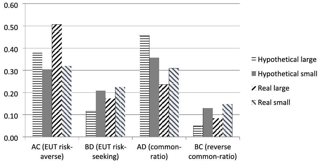
Fig. 2 Frequency of choice patterns for each of four payoff categories—hypothetical payoffs, large and small, i.e., above and below the median hypothetical payoff of $123 (in 2010 USD) and real payoffs, large and small, relatively to the median real payoff of $34 (in 2010 USD)

4 Regression Analysis

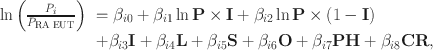
In every experiment each subject can reveal only one of four possible choice patterns: risk-averse EUT-consistent choice, risk-seeking EUT-consistent choice, common-ratio choice pattern, and reverse common-ratio choice pattern. In this case, a multinomial logistic specification is appropriate:

$\begin{array}{cc}ln\left(\frac{P_i}{P_{\text{RA EUT}}}\right)& ={\beta }_{i0}+{\beta }_{i1}lnP\times I+{\beta }_{i2}lnP\times \left(1-I\right)\\ & +{\beta }_{i3}I+{\beta }_{i4}L+{\beta }_{i5}S+{\beta }_{i6}O+{\beta }_{i7}\mathrm{PH}+{\beta }_{i8}\mathrm{CR},\end{array}$

where $P_i$ is the probability of observing a specific choice pattern, i = {risk-seeking EUT, common-ratio, and reverse common-ratio} and risk-averse EUT-consistent choice pattern is set as the baseline outcome and explanatory variables are:

• • highest outcome $P$ (column 11 of Table 1, after conversion to 2010 USD, see footnote 3);

• • real-incentives dummy variable $I$ (column 13 of Table 1);

• • probability of the highest outcome in a risky lottery in the first common-ratio questionFootnote ⁴ $\mathrm{PH}$ (column 9 of Table 1); and

• • the ratio of middle to highest outcome $O$ (column 12 of Table 1);

• • lottery presentation categorical variable $L$ (column 14 of Table 1)Footnote ⁵;

• • student dummy variable S (column 15 of Table 1)Footnote ⁶;

• • the common ratio $\mathrm{CR}$ (column 10 of Table 1).

The highest outcomes $P$ are natural-logged to reconcile a wide range of their values and to reflect saturation. There is a strong negative correlation between $lnP$ and the real incentives dummy variable $I$ , as studies with high payoffs use only hypothetical incentives. We use the interaction terms $lnP\times I$ and $lnP\times \left(1-I\right)$ to allow for different slopes for $lnP$ for the cases of real and hypothetical payoffs, respectively. We also consider several alternative model specifications presented in Table 4 in the supplementary material. (They produce similar results with a lower goodness of fit.)

Table 3 presents the average marginal effects (observation-specific marginal effects averaged over all observations) of the 4-outcome logistic regression (regression coefficients $\beta$ are presented in Table 5 in the supplementary material). Note that average marginal effects for each explanatory variable sum up to zero over the four possible choice patterns. Table 3 reports regular standard errors as well as cluster-robust standard errors. The cluster-robust method allows for correlated residuals within clusters, but not across clusters. Correlations may be induced by some unobserved conditions specific to a cluster. We cluster at the level of the country resulting in 11 clusters.

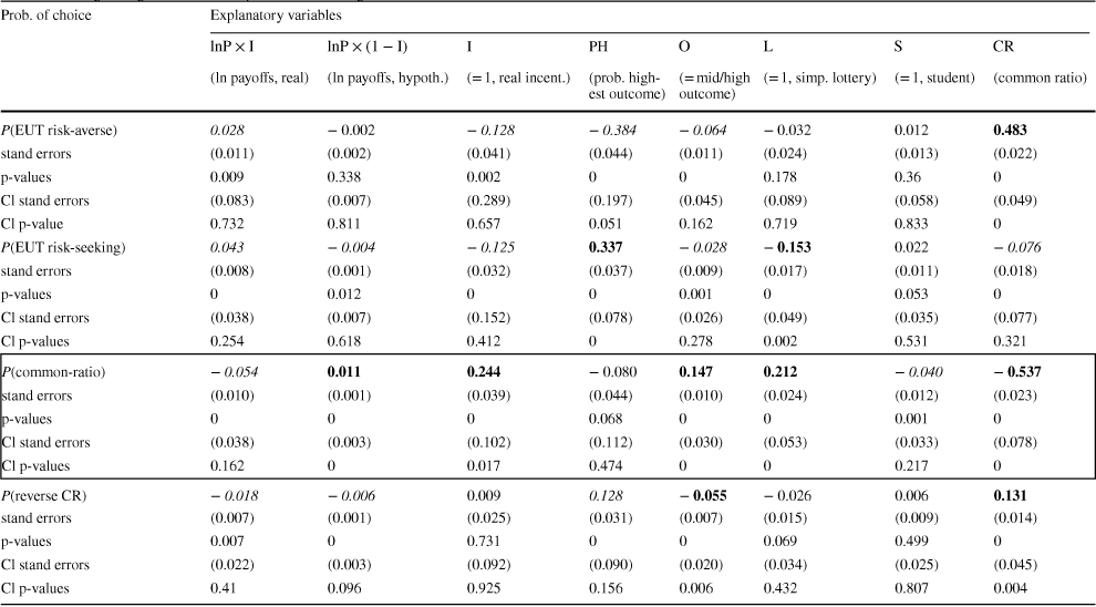
Table 3 Average marginal effects computed from the logit model

Prob. of choice	Explanatory variables
	$\mathrm{lnP}\times I$	$\mathrm{lnP}\times (1-I)$	I	PH	$O$	$L$	$S$	$\mathrm{CR}$
	(ln payoffs, real)	(ln payoffs, hypoth.)	(= 1, real incent.)	(prob. highest outcome)	(= mid/high outcome)	(= 1, simp. lottery)	(= 1, student)	(common ratio)
P(EUT risk-averse)	0.028	− 0.002	− 0.128	− 0.384	− 0.064	− 0.032	0.012	0.483
stand errors	(0.011)	(0.002)	(0.041)	(0.044)	(0.011)	(0.024)	(0.013)	(0.022)
p-values	0.009	0.338	0.002	0	0	0.178	0.36	0
Cl stand errors	(0.083)	(0.007)	(0.289)	(0.197)	(0.045)	(0.089)	(0.058)	(0.049)
Cl p-value	0.732	0.811	0.657	0.051	0.162	0.719	0.833	0
P(EUT risk-seeking)	0.043	− 0.004	− 0.125	0.337	− 0.028	− 0.153	0.022	− 0.076
stand errors	(0.008)	(0.001)	(0.032)	(0.037)	(0.009)	(0.017)	(0.011)	(0.018)
p-values	0	0.012	0	0	0.001	0	0.053	0
Cl stand errors	(0.038)	(0.007)	(0.152)	(0.078)	(0.026)	(0.049)	(0.035)	(0.077)
Cl p-values	0.254	0.618	0.412	0	0.278	0.002	0.531	0.321
P(common-ratio)	− 0.054	0.011	0.244	− 0.080	0.147	0.212	− 0.040	− 0.537
stand errors	(0.010)	(0.001)	(0.039)	(0.044)	(0.010)	(0.024)	(0.012)	(0.023)
p-values	0	0	0	0.068	0	0	0.001	0
Cl stand errors	(0.038)	(0.003)	(0.102)	(0.112)	(0.030)	(0.053)	(0.033)	(0.078)
Cl p-values	0.162	0	0.017	0.474	0	0	0.217	0
P(reverse CR)	− 0.018	− 0.006	0.009	0.128	− 0.055	− 0.026	0.006	0.131
stand errors	(0.007)	(0.001)	(0.025)	(0.031)	(0.007)	(0.015)	(0.009)	(0.014)
p-values	0.007	0	0.731	0	0	0.069	0.499	0
Cl stand errors	(0.022)	(0.003)	(0.092)	(0.090)	(0.020)	(0.034)	(0.025)	(0.045)
Cl p-values	0.41	0.096	0.925	0.156	0.006	0.432	0.807	0.004

We report regular standard errors (in parenthesis), and the cluster-robust standard errors (clustered at the country level). Coefficients significant at 0.05 level for both the regular and cluster-robust methods are highlighted with bold black font. Coefficients significant at 0.05 level for the regular, but not the cluster-robust method are highlighted with italics. (Same convention for Tables 4, 5 in the supplementary material.)

Looking at the probability of observing the common-ratio choice pattern (the section of Table 3 highlighted in boxed text), we find that it is influenced by the following factors. First, a lower common ratio (the last column of Table 3) increases the probability that subjects reveal the common-ratio choice pattern by 0.054 for each 0.1 decrease in the common ratio largely because it decreases the likelihood that subjects reveal the risk-averse EUT-consistent choice. For instance, if we reduce the overall median common ratio of 0.25 to 0.01, as in the original Allais (Reference Allais1953, p. 529) example, the probability of observing the common-ratio choice pattern increases by approximately 0.13. This confirms the well-known observation that experiments with low common ratios produce high instances of EUT violations. We could also speculate that this fact is probably well-known because it happens to be the strongest factor influencing the likelihood of the common-ratio effect.

Second, conducting an experiment with hypothetical incentives increases the chance of observing the common-ratio choice pattern by 0.011 for each relative increase in payoffs (the third column of Table 3). In combination with the intercept term shifter (the fourth column) that is actually lower for the hypothetical incentives than for the real incentives, we conclude that very high hypothetical incentives lead to the increased probability of the common-ratio choice pattern relatively to the low hypothetical incentives. Conversely, for real incentives, the chance of observing the common-ratio choice pattern is reduced by 0.054 for each relative increase in real payoffs. Hence, high real incentives lead to the reduced observations of the common-ratio choice pattern in comparison to low real incentives. This is largely due to the fact that high real incentives increase the likelihood of the EUT-consistent choices (both risk-averse and risk-seeking).

Third, subjects are more likely to reveal the common-ratio effect when choice alternatives are described as simple probability distributions (not in a compound or frequency form), cf. the seventh column of Table 3. Largely this happens because subjects are then less likely to reveal the risk-seeking EUT-consistent choice pattern. For example, changing the presentation format from compound to simple lotteries increases the probability of observing the common-ratio effect by 0.212.

Fourth, designing the common-ratio experiment with the middle outcome being close to the highest outcome (cf. the sixth column of Table 3) favours the instances of the common-ratio choice pattern at the expense of EUT consistent choices and the reverse common-ratio choice pattern. Blavatskyy et al. (2020, Table 2) report a similar effect for the Allais paradox.

Based on our findings we can construct a common-ratio index capturing the main features of the experimental design that favor the common ratio effectFootnote ⁷:

$\text{CRindex}=-0.054lnP\times I+0.011lnP\times \left(1-I\right)+0.244I+0.147O+0.212L+0.537\mathrm{CR}$

Figure 3 plots this index against the share of subjects revealing the common-ratio choice pattern in each of the 143 experimental designs in our data set. The index has predictive abilities.

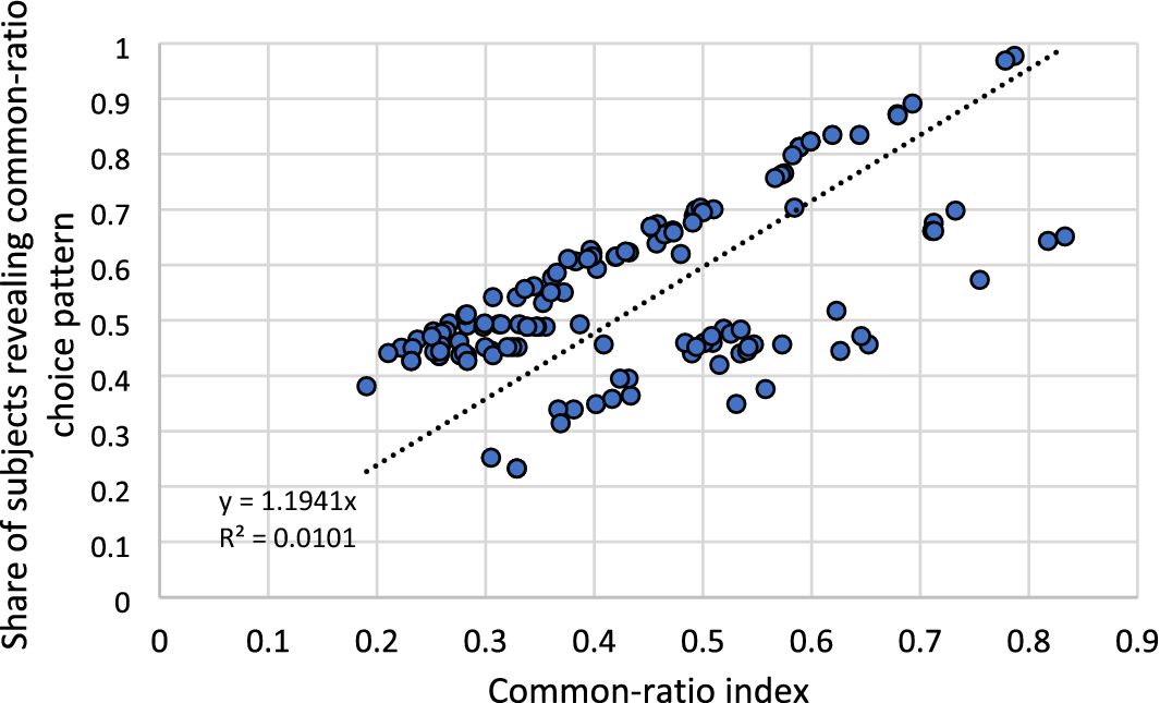
Fig. 3 Share of subjects revealing the common-ratio choice pattern vs. common-ratio index. N = 143 experimental designs. Linear trend is indicated by the dotted line and its equation is reported