


1 Introduction
Substantial research has been devoted to the study of conflict, described as an adversarial interaction between players who expend efforts and try to achieve mutually exclusive goals.Footnote 1 We study dynamic properties of such conflict if the contestants take part in a sequence of pairwise contests, have incomplete information about their opponent’s type and learn from the interactions about the composition of the population of potential future opponents.
Extensive experimental work on conflict confronts theory predictions with subjects’ behavior in the laboratory and has uncovered systematic behavioral departures from the complete information benchmark models. One main interpretation of the findings is that the individuals who interact in conflict games—in the laboratory and elsewhere—follow motives beyond the maximization of monetary payoffs and that these motives are not uniform across individuals. Whereas monetary incentives are typically common knowledge in experimental setups, these other (intrinsic) motivations are not; this turns the interaction into a game with incomplete information. Individuals may know their own preferences but have to form beliefs about the types of opponents they interact with. If players interact repeatedly with other players from the same population (experimental session), they may learn about other players’ types, update their beliefs about the type of future opponents and adjust their behavior accordingly, which may lead to an escalation or de-escalation of contest effort.
The importance of unobserved heterogeneity in individual motivations for behavior in strategic interactions such as conflict games has three main implications, which establish the research agenda of this paper. First, a suitable benchmark model of conflict games needs to incorporate incomplete information about individuals’ ‘preference types’ such as their intrinsic motivation to win. To allow for learning about the population of opponents, the model needs to be dynamic. Second, observed adjustments of behavior in the experimental data should be contrasted with the equilibrium prediction of the dynamic game, which can be structurally different from the complete information benchmark. Third, individual heterogeneity and learning can cause self-selection if the likelihood of future interactions is not fully exogenous such as in models of dynamic conflict that consist of several “battles”.
Our framework adds a simple dynamic structure to a generic model of distributional conflict.Footnote 2 In the multi-stage game considered, each contest stage takes the form of a standard two-player Tullock contest, with the only modification that the prize is awarded with some (exogenous) probability only. Otherwise the game moves to the next contest stage, the players are re-matched in pairs and choose new efforts.Footnote 3 The conflict game is set up such that effects of belief updating and self-selection based on unobserved preference heterogeneity can be isolated in the experimental data. Ignoring preference heterogeneity, a standard theory with complete information (without population uncertainty) would predict behavior to be identical across all stages of conflict. This is mainly due to the assumption of an exogenous continuation probability which, hence, plays a key role for the identification strategy by removing the strategic links between the stages, except possibly for belief updating.Footnote 4
Unobserved heterogeneity in characteristics such as the intrinsic motivation to win and uncertainty about the composition of the population of opponents introduce dynamics of conflict behavior caused by belief formation and updating. In line with a theory of social projection, we show that a player’s own preference type partially shapes her beliefs about other participants.Footnote 5 The different player types start with different beliefs about the population of opponents. Learning about the opponents’ propensity to exert effort has different strategic implications for players who are strongly or weakly intrinsically motivated. Intuitively, learning that a majority of opponents have a weak intrinsic motivation (choose low effort) reduces the incentive to exert effort for strongly motivated participants, as they can ensure a high win probability at lower costs. However, the same signal about the opponents increases the incentive to exert effort for weakly motivated participants, similar to an encouragement effect. This logic is closely related to strategic considerations in other contest applications and is a consequence of the usual non-monotonicity of best reply functions.
In the closely corresponding baseline experimental treatment (BASE), a monetary prize is awarded based on a Tullock function with probability 1/3 in a given stage, which would end the game. In each stage reached, the players are randomly matched in pairs and, apart from choosing contest expenditures, have to state their beliefs about the opponent’s effort. If the prize has not been awarded after 5 stages, the game ends without prize allocation. We find considerable evidence for nonincentivized heterogeneity among players which—together with the implied updating of beliefs in later stages—also explains dynamic adjustments of contest efforts across the contest stages. Unobserved preference heterogeneity and belief formation about potential opponents are seemingly a driver of the observed effort escalation and de-escalation; not allowing for this type of information asymmetries would yield theory predictions that are structurally different from the experimental findings.
As a main experimental variation (the EXIT treatment), we consider a variant of the game that allows for self-selection—an aspect which is crucial in most dynamic conflict games where participation at later stages is not fully exogenous.Footnote 6 To emphasize the implications of self-selection in the presence of unobserved preference heterogeneity, we extend the multi-stage contest by an explicit continuation decision after the first contest encounter (to be made in case the prize has not yet been awarded). The outside option is chosen such that equilibrium behavior based on monetary payoff maximization does not change, that is, it is lower than the equilibrium expected continuation payoff. The experimental results, however, confirm our theory prediction that unobserved preference heterogeneity and updating about the population of future opponents can cause self-selection of certain types into continuing conflict and result in an escalation of efforts in later contest stages.
Our paper is the first to develop and test a theory of sequential contests in which conflict behavior may be driven by intrinsic (behavioral) motives, in which players cannot observe the intensity of the motives of their competitors, and in which they are uncertain about the environment described by the distribution of types of possible competitors. While the dynamics of conflict caused by population uncertainty and belief updating have not been studied, some elements of this theory relate to results that have been developed in the theory of all-pay contests with incomplete information in a purely static context. Malueg and Yates (Reference Malueg and Yates2004) analyze the static contest between two players whose prize valuations are drawn from a commonly known binary distribution. Even though their information assumption differs from the one that emerges from social projection in our dynamic framework, their results are structurally similar to stage 1 of our game. Fey (Reference Fey2008), Ryvkin (Reference Ryvkin2010), Wasser (Reference Wasser2013a, Reference Wasserb) and Einy et al. (Reference Einy, Haimankoa, Moreno, Sela and Shitovitz2015) study existence of Bayesian equilibrium in the static incomplete information Tullock contest.Footnote 7 The results by Einy et al. (Reference Einy, Haimankoa, Moreno, Sela and Shitovitz2015) are closest to our existence results, as they allow players to have private information about the state of nature.
Broad empirical evidence on conflict behavior suggests an intrinsic motivation to win, leading to a mismatch between a complete information benchmark and the experimental results. Moreover, contest efforts often exhibit dynamics that do not square with the standard theory intuition.Footnote 8 Other findings suggest that self-selection based on unobserved heterogeneity of contestants may explain deviations from the complete information benchmark model. In line with this, Fu et al. (Reference Fu, Gürtler and Münster2013) show that players sometimes engage in costly messages prior to a lottery contest and explore the role of incomplete information as the rationale for this behavior. Herbst (Reference Herbst2016) finds selection effects which she explains by players’ differences in a ‘joy of winning’. Herbst et al. (Reference Herbst, Konrad and Morath2015) consider unobserved behavioral heterogeneity of players in the context of free-riding in fighting alliances and the endogenous versus exogenous formation of such alliances. They also find that players make inference from past actions of their co-players, and weak players exploit strong players if both types enter into the same fighting alliance. Strong players understand this and tend to self-select: rather than joining the fighting alliance with a player who is likely to be weakly motivated, they prefer to become stand-alone fighters. In our paper, random re-matching after each interaction avoids that players can make inference on the behavioral type of their specific co-player. However, the players learn about the nature of the overall population. This population learning turns out to be sufficient for an adjustment of their behavior and for whether to continue to participate in the conflict game or quit.
Another dimension of learning dynamics in experimental contests concerns the extent to which feedback is provided, with mixed evidence so far. In a setting with fixed matching of participants, Fallucchi et al. (Reference Fallucchi, Renner and Sefton2013) find that information about the opponent’s choice has opposite effects on effort levels in probabilistic and deterministic contests. Mago et al. (Reference Mago, Samak and Sheremeta2016) consider four-player contests with fixed matching and find no effect of information about others’ effort on average efforts but dynamic adjustments of efforts which reduce effort heterogeneity (the latter is in line with our theory; the former may arise from the predicted countervailing adjustments of different player types). Keeping the set of choices observed at each stage constant and eliminating learning about the specific opponents and hence strategic signaling by design, our approach addresses the idea that different types of players may hold systematically different beliefs, which can lead to different adjustments of beliefs and efforts when learning about the population of potential opponents.
Our paper also relates to a methodological discussion of the benchmark choice in laboratory experiments. If players understand that their co-players do not play the money-guided Nash equilibrium action, this should trigger a different optimal reply, even for strictly money-oriented players. Fudenberg and Levine (Reference Fudenberg and Levine1997) find evidence in experimental contexts that actual co-players’ behavior may induce learning and may cause players to optimize against this observed behavior. Konrad et al. (Reference Konrad, Morath and Mueller2014) report similar findings in the context of monopoly pricing and consumer boycott. Camerer and Weigelt (Reference Camerer and Weigelt1988) study experimental behavior in a finite lending game with reputation building. In their context, players have incomplete information about other players’ monetary incentives by experimental design of the game. Our approach combines elements of these approaches. We do not induce heterogeneity in incentives or incomplete information about these incentives. We rather draw on experimental evidence that finds players’ heterogeneity along an important (‘behavioral’) dimension and acknowledge that subjects have incomplete information about the non-monetary payoff components of their opponents.Footnote 9
The role of population uncertainty, self-projection and Bayesian learning may be important in various contexts beyond contest applications. Ample evidence has shown that many players who interact in a laboratory environment have motives in addition to the extrinsic monetary incentives provided.Footnote 10 Since players cannot really know the distribution of types in a subject pool when taking part in an experiment, a well-reasoned choice requires players who enter a laboratory session to form a belief about the composition of the population of subjects from which the co-players are drawn. It may be appealing early on to make Bayesian inference from one’s own type and update this belief from interaction to interaction. With an increasing number of observations of others’ choices the importance of a player’s own type for the beliefs about the opponents’ types may fade.
2 Theoretical framework
2.1 Model
We consider a framework in which conflict about a prize takes place in up to n stages, each described as a Tullock contest. The players differ in their prize valuation and there is uncertainty about the probability distribution of types. The theory framework allows for learning about the true type distribution but, by construction, removes strategic aspects of how own effort choices are interpreted by others. One variant of the analysis allows for players’ selection by including the possibility to exit the multi-stage game.
Players, actions, and timing Let I be an infinitely large set of players. The game has up to n stages but may end before reaching the terminal stage. In any given non-terminal stage
 , if this stage is reached, each player i is randomly matched with one other player
 . Players i and
 simultaneously choose efforts
 and
and
 , where
 . This leads to one of three outcomes, described from the point of view of player i. In the first outcome i wins a prize and reaches no further stage (that is, the game ends for i). In the second outcome player
 wins this prize; again, i reaches no further stage (the game ends for i). In the third outcome none of the two players wins the prize but the game continues for i who enters stage
 . This third outcome emerges with probability
 . This probability is exogenously given and does not depend on
 or
or
 . The other two outcomes emerge with probabilities
 and
and
 . As will become clear below, the assumption of an exogenous continuation probability
 is the key assumption that allows to isolate selection effects in the experimental data.
The function
 describes the win probability of player i in stage s, conditional on the prize being awarded in this stage. This conditional probability is a function of the player’s own effort and the opponent
 ’s effort at this stage. We assume that this function is given by the Tullock (Reference Tullock and Buchanan1980) contest success function:
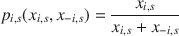
for all stages
 .Footnote 11 The function
 is continuous, strictly increasing and concave in player i’s own effort and strictly decreasing in the effort of the opponent
 of this stage.Footnote 12
If the prize is not allocated in stage
 such that player i enters into stage
 , the players are randomly re-matched. Hence, the identity of the opponent typically changes between stages, as the set I of players is infinitely large. We denote by i a given player (with unchanged identity over all stages that are reached) and by
 the opponent assigned to player i in a given stage. In stage
 , player i and the new opponent
 choose efforts
 and
and
 and the stage contest resolves according to the same rules as in stage s. This continues until the game ends for i because one of the players wins the prize, or until the terminal stage
 is reached. Interaction at the terminal stage n follows the same rules as in previous stages, with one difference: should none of the two players win at stage n , the game ends and no prize is awarded.
Payoffs Payoffs consist of the prize value if the player wins, minus the own effort costs that are ‘all pay’: Players i and
 pay the cost of their own efforts
 and
and
 . By normalization, these costs are equal to
 and
and
 . They occur independent of whether or not a player wins at stage s, or whether the prize is awarded in this stage at all. There is no discounting, so effort costs add up for the different stages.
Player i values winning the prize by
 , which is private information. This fact and the probability model that describes the random process behind the assignment of valuations is common knowledge and formalized below. Player i learns her own prize valuation
 prior to the first effort choice in stage 1. We assume that a player keeps this valuation of winning throughout all stages of the game. Players may differ in their valuation of the prize: one share of players has a valuation
 , the other share of players has a valuation
 .Footnote 13 We sometimes call a player with valuation
 a ‘weak’ player and a player with valuation
 a ‘strong’ player. As there is no discounting, a player has the same benefit from winning the prize if she wins at stage s as if she wins at stage
 .
.
Altogether, player i’s payoff is
 if i wins the prize at stage s,
 if
if
 wins the prize at stage s, and
 if the prize is not allocated at any stage
 .
.
Population uncertainty and information structure The prize valuation
 is assigned to player i in a random process that has two layers of randomness. First, there are two possible states of the world that may prevail. These states
 and
and
 differ in the probability distribution from which the players’ valuations are drawn. All players start with common prior beliefs
 about the probability that the world is in state
 and attach a probability of 1 / 2 to each of the two possible states.
Second, nature draws the type of each player
 independently from the same given probability distribution, which depends on the state of the world. Specifically, in state
 of the world, player i is assigned valuation
 with probability
 , and is assigned valuation
 with the complementary probability
 ; we assume that
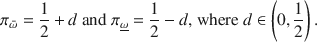
Hence, the state of the world characterizes the share of high types,
 , and the share of low types,
 , in the population; the share of high types is larger in state
 than in state
 . For
. For
 the player’s own type as well as the experienced opponents’ efforts affect the players’ updating about the probability for the world to be in state
 or
or
 .
.
Beliefs At the beginning of stage 1, each player
 learns her valuation
 , which i keeps throughout the game. As
 is a random draw from the true probability distribution (which is one of two possible ones), this makes i’s own valuation not only important for the payoff from winning but also for the beliefs about other players’ valuations: player i uses Bayes’ rule to update her belief about the true state of the world, which is then used to determine her beliefs about the composition of the population from which the opponent
 is drawn. In stages
 (if reached), the beliefs also depend on the history of opponents’ efforts in previous stages
 .
.
Formally, in stage s the population is composed of players with different prize valuations
 and different histories of observed efforts of previous opponents
 ; the vector

describes all relevant information about a player’s genuine type (prize valuation) and experience type (history of opponents’ effort choices) at the beginning of stage s. Somewhat loosely we refer to
 as i’s ‘type’ in stage s where
 denotes the set of types in stage s. For a player i of type
 to be teamed up with player j of type
 , the probability beliefs are characterized by cumulative distribution functions
 . Atoms in these distributions will be denoted by
 ; they measure the probability which a player i with valuation
 and experienced opponents’ effort
 attributes to the event that her newly matched opponent
 in stage s has a prize valuation
 and experienced previous opponents with expenditures
 .
.
2.2 Benchmark: no uncertainty about the state of the world
Before analyzing the model with population uncertainty and Bayesian updating, we consider a benchmark case for which the true state
 is common knowledge and player types are independently drawn from the respective distribution in which
 is the known share of players with valuation
 .
.
Proposition 1
Suppose that there is common knowledge about the share
 of high-valuation players and denote the equilibrium efforts by
 and
and
 for players with valuation
 and
and
 , respectively. Then,
 and
and
 are constant across all stages
s
that are reached. All player types expect that their rival’s
effort is, on average,
are constant across all stages
s
that are reached. All player types expect that their rival’s
effort is, on average,

The proofs of this and all subsequent propositions are in Appendix 1. In the benchmark of a known distribution of types, a player cannot learn from her own type or other players’ effort about future opponents’ types. Thus, each of the stages can be seen as independent; the dynamic game can be interpreted as a sequence of completely independent static games.Footnote 14 An interior equilibrium

 at a given stage is described by the first-order conditions
and
The equilibrium levels of a player are precisely the same in each stage s and the players’ expectations of the rival’s effort are independent of the own player type.
Special parametric cases have been solved explicitly in the literature. If
 , the first-order conditions become
[as in Malueg and Yates (Reference Malueg and Yates2004)]. For the case of symmetric players with
 , this solution reduces to
 , which corresponds to the result obtained by Tullock (Reference Tullock and Buchanan1980).
2.3 Perfect Bayesian equilibrium with learning
This section contains the theory results for the framework with uncertainty about the distribution of types. We show existence of a perfect Bayesian equilibrium of the dynamic game and offer a partial characterization of the equilibrium efforts.
Proposition 2
A perfect Bayesian equilibrium in pure strategies exists.
In each stage, players form beliefs about the composition of the set of players conditional on their own valuation and the behavior of players they have previously been matched with. The equilibrium beliefs at each stage are characterized by finite sets of mass points
 . Based on these the players maximize their expected payoff in the contest of the respective stage. Compactness and continuity properties of the optimal choices allow us to apply Brouwer’s fixed point theorem to conclude that this class of problems has a fixed point that characterizes an equilibrium of the static Bayesian game at each stage.
The linkage between stages is via belief updating about the composition of the set of possible opponents. Random re-matching of players at each stage and the size of the set of possible opponents become important here, causing that player i’s effort choice at a given stage only affects the future beliefs of a finite number of other players that form a set of zero probability mass. From a single player’s perspective this turns the problem into a sequence of structurally independent Bayesian games.
Stage 1 properties At the beginning of stage 1, the players’ beliefs depend on their own valuation only, that is, types
 .
.
Lemma 1
In stage
 , players with valuation
 and
and
 , respectively, believe that the share of high-valuation players in the population is given by
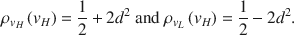
Using straightforward Bayesian updating, the beliefs in (7) are derived in two steps. First, type
 updates her beliefs
 about the probability that the true state of the world is
 . The beliefs about the share of high types in (7) follow directly from
 and Bayes’ rule. As (7) shows, each player believes that the state of the world is more likely in which the player’s own type is more likely, and thus believes that it is more likely to face an opponent of the same type. Lemma Footnote 1 can explain if players of different types form different beliefs about their opponent’s type and, hence, effort in the first stage. The next proposition characterizes explicitly the stage 1 equilibrium efforts
 and the players’ expectations
 about their opponent’s effort.
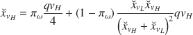
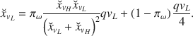
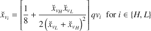
Proposition 3
Denote the equilibrium efforts in stage 1 by
 and
and
 for players with valuations
 and
and
 . If
. If

 , these efforts are equal
to
, these efforts are equal
to
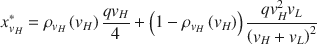
and
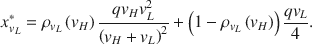
Equilibrium beliefs about the opponent’s expected effort are

and

with

In the stage 1 contest, the equilibrium effort of a player of type
 turns out to be a weighted average of the efforts in the corresponding complete information contests in which the valuations of winning are commonly known, that is, for valuations
 . A comparison of
 and
and
 in (8) and (9) with
 and
and
 as in (5) and (6) shows that subjective probabilities
 and
and
 of facing a high-valuation player replace the objective probability
 . Since
 , strong types place more weight on the possibility that
 is a strong type as well, and vice versa. These different weights generate the two different conjectures (10) and (11) about the expected effort of the opponent. This contrasts with the type-independent expectations in Proposition Footnote 1.
It is known that it is difficult to solve analytically for the equilibrium of the Tullock contest with incomplete information. Only partial results exist in the literature.Footnote 15 The equilibrium described in Lemma Footnote 1 and Proposition Footnote 3 considers the case of players who are drawn from the same distribution but can differ in their beliefs about the underlying distribution of types, as a consequence of uncertainty about the true type distribution. A further comparative static result is stated as a corollary.Footnote 16
Corollary 1
The stage 1 equilibrium effort
 of strong types is strictly increasing in
 and the stage 1 equilibrium effort
 of weak types is strictly decreasing in
 .
.
This result is in line with standard intuition in contest theory: players exert more effort if they believe it is likely to meet another player with the same (a similar) valuation. Thus, if strong types believe that it is more likely to be in state
 (with many strong types) they adjust their effort upward. If weak types believe that it is more likely to be in state
 they adjust their effort downward. With (7), both types’ efforts in stage 1 go up if the distance d between the two possible states of the world is increased. A higher value of d implies that the true type distribution is more asymmetric; hence, stage 1 beliefs react more strongly to the information about the own type and players expect their opponent to be of the same type with higher probability.
Later stages In stages
 , player i’s ‘type’ is characterized by the own prize valuation and a history of encounters with other players
 with their own valuation
 and history of previously matched players. If
 contained already m different player types, then any player can be matched with any of these types, such that the set
 contains
 elements. In Section B.1 of the Online Appendix we consider properties of stage
 and establish a ranking of equilibrium efforts (Proposition 6) that demonstrates the potentially countervailing effects of valuation type and experience type on incentives to exert effort. Proposition 6 in the Online Appendix also shows that the stage 2 equilibrium beliefs about the opponent’s effort satisfy

where, in the subscript, the first element refers to the player’s own valuation and the second element refers to the effort of the stage 1 opponent. Hence, a player’s expectation of the opponent’s effort is still correlated with the own valuation type so that high-valuation players expect, on average, higher opponent’s effort than low-valuation players.
It is evident that calculating the equilibrium efforts for this problem becomes increasingly intractable in later stages. However, we can consider a limit case where the maximum number of stages grows very large and discuss changes in beliefs and efforts across the stages on an intuitive basis. If the opponents’ effort choices remain informative about the type distribution, the impact of the own type on the players’ beliefs in stage s becomes less and less important in later stages, as the number of signals obtained increases rapidly (the opponent’s effort in stage s is not only informative about this opponent’s valuation but also about the opponent’s experience in previous stages). In the limit case after a sufficient number of stages, the heterogeneity in beliefs should disappear and all players’ beliefs about the share of players with a high prize valuation should converge to the true share
 (where
 ).Footnote 17 Moreover, the players anticipate that their opponent will have the same beliefs with probability (close to) one. As a consequence, the correlation between a player’s own effort and the average effort she expects from her stage s opponent identified in (12) and (13) above vanishes in later stages:

Similarly, the average equilibrium effort of high-valuation (low-valuation) players converges to the equilibrium effort of high-valuation (low-valuation) players in a contest in which the players have common beliefs about the type distribution.
To shed light on the expected direction of effort adjustments of strong and weak types, we compare the stage 1 equilibrium efforts
 and
and
 given in (8) and (9) to the equilibrium efforts in “very late” stages, where the true share of high types is (basically) common knowledge as in Proposition Footnote 1. The latter are denoted by
 and
and
 and we assume an interior equilibrium

 .
.
Proposition 4
(i) If the state of the world is
 (with many strong types), then
 . (ii) If the state of the world is
 (with many weak types), then
 and
and
 .
.
Proposition Footnote 4 provides a further theoretical foundation for the empirical analysis below. In particular, it makes a prediction on the adjustments of efforts of low and high types in late stages as compared to stage 1 conditional on the shape of the type distribution. More informally, if the true distribution of types is such that there are many low-valuation players, the players’ beliefs about the share of strong types are corrected downwards in later stages as compared to the players’ beliefs at stage 1. This holds in particular for high-valuation players who initially believe that there are more strong types (compare (7)). As a consequence of this updating, the average effort of strong types should be decreasing and the average effort of weak types should be increasing in later stages. Conversely, if the distribution of types is such that there are many high-valuation players, the average effort of strong types should be increasing and the average effort of weak types should be decreasing in later stages.Footnote 18 These different dynamics reflect the intuition that players increase their effort if they learn that it is likely to face an opponent with a similar valuation, and reduce their effort if they learn that the contest is likely to be asymmetric.
An exit option and self-selection In order to identify selection effects in the data, a modified version of the game allows players to exit the game at the end of stage 1 in case the conflict has not yet been resolved. Formally, after observing the outcome of the stage 1 contest, all players simultaneously and independently decide whether to exit the game. In case of exit a player receives a fixed payment b but does no longer participate in stages
 . For the players who do not exit the game continues with possible contest stages
 within the population of players who did not exit. If all but a set of players with mass zero exit, the game ends for all players.
Proposition 5
Suppose that exit is possible at the end of stage 1. For an exit payment
 , there is a perfect Bayesian equilibrium in which all players with valuation
 exit and all players with valuation
 do not exit, where
 and
and
 are given by

with
 and
and

At stages
 (if reached), all players believe that their opponent has a valuation
 with probability one and equilibrium efforts are equal to

For intermediate values of the exit option, there is an equilibrium in which all weak types exit so that the population of players in stages
 consists of strong types only. The value
 represents the expected continuation payoff of strong types; the constraint
 ensures that weak types do not want to deviate from this equilibrium.Footnote 19
In the equilibrium in which weak types exit and strong types remain, average effort in stages
 is strictly higher than average stage 1 effort, due to two effects.Footnote 20 First, there is the direct self-selection effect that causes the population in stages
 to be composed only of players who care strongly about winning. Second, since in stages
 strong types correctly anticipate that their opponent will be a strong type, they further increase their effort as compared to stage 1.
2.4 Summary of the main predictions
The theoretical analysis provides the basis of four main testable predictions. First, ignoring potential type heterogeneity and population uncertainty, efforts should be constant across all stages and beliefs should be type-independent (Proposition Footnote 1). Second, if there is unobservable heterogeneity in the (intrinsic) motivation to win and players are ex ante uncertain about the distribution of these player types in the population, then the individual beliefs about the opponent’s effort are positively correlated with the own effort in early stages of the game. The correlation should become weaker in later stages of the game (compare Lemma Footnote 1 and Proposition 6 in Section B.1 of the Online Appendix as well as the discussion around (14)). Third, if the true type distribution consists of more weak types than expected (with a low intrinsic motivation), weak types’ effort should go up and strong types’ effort should go down in later stages, as compared to stage 1 (Proposition Footnote 4). The opposite dynamics should prevail if the population consists of more strong types than expected. Forth, if exit is possible at the end of stage 1, weak types should exit and strong types should remain so that average effort in stages
 is strictly higher than average stage 1 effort (Proposition Footnote 5).
The intuition for the dynamics of efforts closely follows a standard contest logic which is due to the non-monotonicity of best-reply functions. Weak types should be discouraged when learning that there are many strong opponents, and encouraged when learning that there are many weak opponents. Strong types should become more competitive when learning that there are many strong opponents, and should be “appeased” when learning there are many weak opponents. Together with the direction in which the beliefs are adjusted in the respective population, this explains the basic mechanism behind Proposition Footnote 4.
3 Experimental design
To emphasize the importance of accounting for unobserved type heterogeneity, the experimental treatments use the common approach of symmetric monetary incentives (a given contest prize) and common knowledge about these. As explained above, however, we expect significant preference heterogeneity even under symmetric monetary incentives. Thus, our experimental strategy picks up on naturally occurring heterogeneities (as present in most experiments) in order to contrast the structurally different theory predictions with and without incomplete information and population uncertainty.
3.1 Treatments
The baseline experimental treatment BASE corresponds to the theory framework outlined above and investigates the importance of accounting for unobserved heterogeneity in preference types and belief formation, as opposed to the benchmark prediction based on complete information. In the experiment, the individuals compete in up to
 stages about a prize of monetary value
 by choosing investments
 from the set
 at each stage s that is reached. Together with the choice of the own effort, each individual has to state the effort she expects from her opponent at this stage (as a number between 1 and 450); the stated beliefs
 are not displayed to other players. After the effort choices have been made at stage s, the individuals observe the investment
 of their opponent and a “lottery wheel” determines whether one of the two players is allocated the prize or whether the game proceeds to the next stage; this outcome is observed, too.Footnote 21 The exogenous probability that the prize is allocated in a given stage is
 , which is supposed to balance a reasonable chance of winning the prize with a sufficiently high probability of continuation and, hence, possible dynamics. At each stage, the individuals are randomly re-matched in pairs. Once the game ends because the prize has been allocated or stage
 has been completed without prize allocation, each individual is displayed her own payoff.
This design with random matching as well as anonymity and non-identifiability of participants stays close to the theory as long as the subjects in the laboratory do not believe that their actions have informational content that feeds back into their own future encounters. The probability that, in a given session, a player interacted with the same player more than once is not zero in our setup, but the respective player would not know if/when meeting a particular opponent again, which should make quasi-repeated play effects rather unlikely.
Whereas dynamic conflict games typically involve explicit or implicit participation decisions, the BASE treatment removes such considerations by design. As the main experimental variation, the EXIT treatment therefore adds the possibility of exit and, hence, an explicit continuation decision. Based on this experimental variation, we can identify possible effort escalation caused by self-selection as a consequence of unobserved preference heterogeneity. As in the modified theory framework described above, the individuals have the option to exit the game at the end of stage 1, after observing the stage 1 efforts and outcome and in case the prize has not yet been allocated at stage 1.Footnote 22 Individuals make this choice between “exit” and “remain” simultaneously and independently. Denote the stage 1 pair of players by
 . If both i and
 choose to exit then the game ends for both individuals with an exit payment of 60 points each (minus the individual cost of stage 1 effort). If both individuals i and
 choose to remain then both enter into stage 2 (where new pairs of subjects are randomly formed). If one individual chooses to exit and her stage 1 opponent chooses to remain then a coin flip decides on whether both subjects exit or enter into stage 2.Footnote 23 Apart from adding this exit option, the sequence of actions in the EXIT treatment is exactly as in the BASE treatment. The payment in case of exit is chosen to be lower than the equilibrium expected continuation payoff in the benchmark case with symmetric players who maximize their monetary payoffs so that in the latter case no player should exit in equilibrium.
Our choice of symmetric monetary incentives allows to attribute any heterogeneity in behavior to differences in unobserved (preference) characteristics. This comes at the cost of not being able to identify different types of players based on an observable objective function but having to rely on individual choices in order to distinguish different behavioral types of players. This latter approach to classifying types, which is common when one expects factors beyond monetary payoffs to matter, would be appropriate even when imposing heterogeneity in extrinsic (incentivized) motivations as another layer of heterogeneity: even with imposed differences in effort costs, for instance, the sets of individuals with identical monetary incentives would have to be expected to differ along important preference characteristics. The vast majority of contest experiments has shown that behavior cannot be understood without incorporating motives beyond monetary payoff maximization.Footnote 24
3.2 Experimental procedures
The experiment was conducted at econlab Munich in two waves and 19 sessions in total (with typically 24 subjects per session). A first wave in April 2016 involved 4 sessions of each treatment BASE and EXIT; in this wave, the elicitation of beliefs was not incentivized to reduce complexity. A second wave in May 2019 involved 4 sessions of the BASE treatment for which the elicitation of beliefs was incentivized, plus 4 BASE sessions with nonincentivized beliefs and 3 EXIT sessions to ensure comparability of the two waves. The subjects (422 in total) were typically students of Munich universities.Footnote 25 Each subject took part in exactly one session. In each treatment, the respective multi-stage contest was played for 15 times. In other words, each subject played the same game (with up to 5 stages s) in 15 rounds r.
At the beginning of each session each subject was shown a video on the computer screen in which the experimental instructions (also distributed as hard copy) were read aloud. Then, the subjects had to answer a few control questions to ensure they understood the rules of the experiment. After the 15 rounds of the main experiment, we conducted an extended post-experimental questionnaire which, apart from socioeconomic information and questions about the experiment, elicited measures for risk preferences, distributional preferences, ambiguity aversion, loss aversion, and cognitive reflection. At the end of the experiment, 3 out of the 15 rounds were randomly selected for payment and a subject’s total points won minus her investments
 were summed up. In the sessions in which the stated beliefs were incentivized, one further round was selected (different from the 3 rounds for which the contest outcome was paid) and a subject obtained 450 points if her stated beliefs in this additional round deviated, on average, by 5 points or less from the actual opponent effort (that is, if on average
 in this round). Moreover, one of the incentivized post-experimental tasks were randomly selected for payment. The resulting amount of money was converted to Euros at the rate 50 : 1 and added to (or subtracted from) an endowment of 10 Euros. On average a session lasted 90 minutes and the average payment was 17.70 Euros plus a show-up fee of 6 Euros.
For the experimental sessions, the randomization of whether or not in a given stage
 of round
 the prize would be allocated (with the exogenous probability
 ) was conducted (but not announced) before the start of the first session and was kept the same across all treatments, sessions, and subject pairs.Footnote 26 In other words, the number of stages to be played within round
 was the same for all subjects. This ensures that learning about the game and the numbers of signals obtained about the distribution of types are identical across treatments and sessions at any stage s of round r. The random re-matching took place in subgroups (typically 8 subjects, although the precise size of the matching groups was not made explicit) in order to gain more independence of observations and allow us to investigate learning dynamics across different populations.Footnote 27
4 Results
4.1 Overview of the main results
Do the individuals adjust their effort in later stages of the game, and if yes, is there a tendency to escalate or to de-escalate for different player types? The left panel of Fig. 1 provides a first answer to this question by plotting average efforts in the five stages. The graph shows that in the BASE treatment there is a slight upward trend in average efforts. In the EXIT treatment, stage 1 efforts are comparable, but from stage 2 onward (after exit was possible) there is an upward jump in average efforts (in line with Proposition Footnote 5). The higher variance in efforts in the EXIT treatment may be caused by the lower number of observations in stages 2–5 (due to exit of a substantial share of individuals).
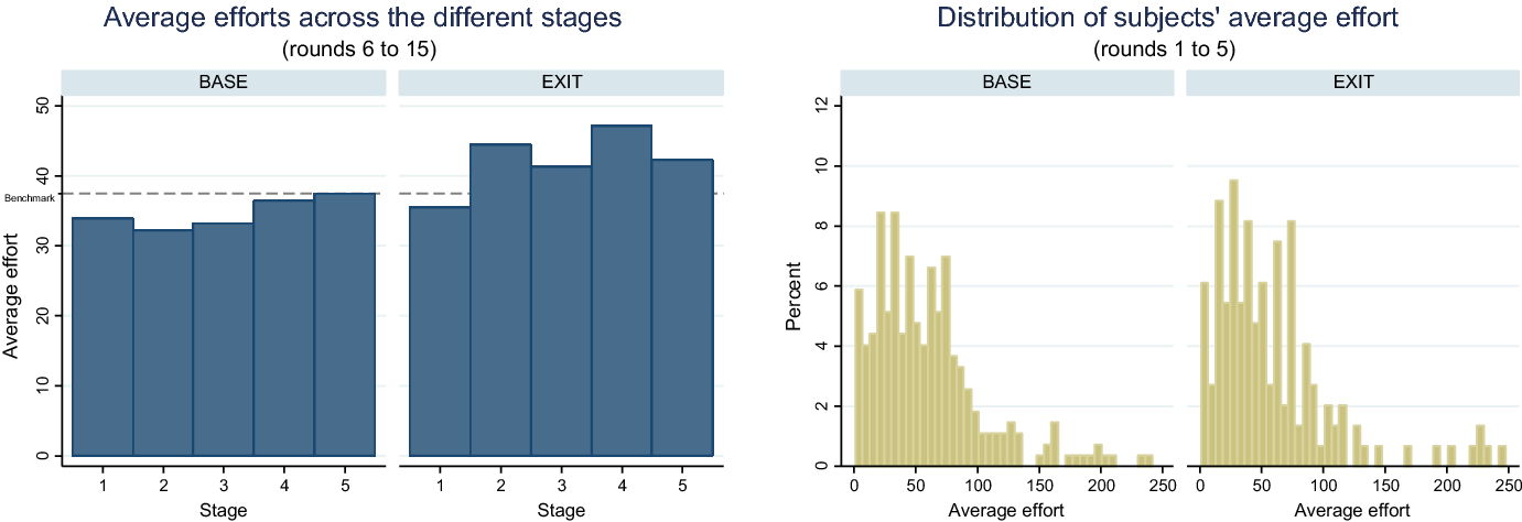
Fig. 1 Left panel: average effort choices in stages 1–5 by treatment; right panel: distribution of ‘types’ by treatment
A regression analysis confirms the finding suggested by the left panel of Fig. 1: we can reject the complete-information prediction of Proposition Footnote 1 (the prediction ignoring population uncertainty) that average efforts do not change across the treatments, even when disregarding possibly different dynamics of different player types. Table 3 in Section B.3 of the Online Appendix summarizes the corresponding results from a set of random-effects regressions based on individual efforts, which estimate the average change in efforts across the stages.Footnote 28
Result 1
Average efforts significantly change across the stages, in contrast to the complete-information benchmark. The effect is strongest in the EXIT treatment where average efforts go up by
 after exit was possible.
The right panel of Fig. 1 reveals a considerable heterogeneity in individual behavior by plotting the distribution of the individuals’ average effort choice in early rounds (rounds 1–5). Accounting for this evident, nonincentivized heterogeneity, which is a common finding in contest experiments, we turn to the main analysis of type-dependent effort adjustments. Since the data from the two different waves of the experiment yields identical conclusions, the subsequent analysis pools the sessions from the two waves.
4.2 On individual efforts
Whereas the theory above makes no definite statement about average adjustments of efforts, it predicts differential effects for different ‘types’ of players with different intrinsic motivations: players classified as ‘weak’ and players classified as ‘strong’. To allow for such (unobserved) heterogeneity we use an individual’s effort choice as a proxy for her valuation of winning. We separate the individuals into strong and weak types according to whether their average effort in rounds 1–5 (as plotted in the right panel of Fig. 1) is below or above the treatment average in those rounds.Footnote 29 With this classification as weak or strong type, we estimate efforts
 (of individual i in stage s of round r) across the stages based on the data of rounds 6–15, interacting the main explanatory variables “Stage
 ” and
” and
 , respectively, with the proxy for a player’s type (an indicator variable
 ). The variable “Stage
 ” is equal to
 so that the coefficient of “Stage
 ” measures the average per-stage change in effort and the intercept estimates average effort in stage 1. The indicator variable
 for the observations from stages
 identifies an effect of the exit option in the EXIT treatment.
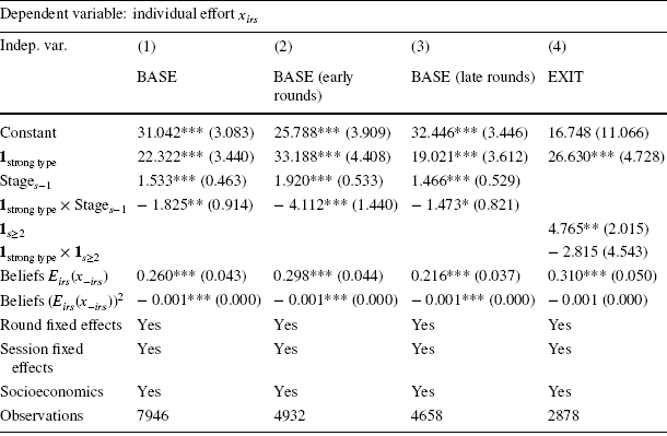
Table 1 Individual effort over stages 1–5: strong versus weak types
|
|
||||
|---|---|---|---|---|
|
Indep. var. |
(1) |
(2) |
(3) |
(4) |
|
BASE |
BASE (early rounds) |
BASE (late rounds) |
EXIT |
|
|
Constant |
31.042*** (3.083) |
25.788*** (3.909) |
32.446*** (3.446) |
16.748 (11.066) |
|
|
22.322*** (3.440) |
33.188*** (4.408) |
19.021*** (3.612) |
26.630*** (4.728) |
|
|
1.533*** (0.463) |
1.920*** (0.533) |
1.466*** (0.529) |
|
|
|
− 1.825** (0.914) |
− 4.112*** (1.440) |
− 1.473* (0.821) |
|
|
|
4.765** (2.015) |
|||
|
|
− 2.815 (4.543) |
|||
|
Beliefs
|
0.260*** (0.043) |
0.298*** (0.044) |
0.216*** (0.037) |
0.310*** (0.050) |
|
Beliefs
|
− 0.001*** (0.000) |
− 0.001*** (0.000) |
− 0.001*** (0.000) |
− 0.001 (0.000) |
|
Round fixed effects |
Yes |
Yes |
Yes |
Yes |
|
Session fixed effects |
Yes |
Yes |
Yes |
Yes |
|
Socioeconomics |
Yes |
Yes |
Yes |
Yes |
|
Observations |
7946 |
4932 |
4658 |
2878 |


Random-effects regressions; SE in parentheses, clustered at the level of matching groups; *** (**, *) significant at 1% (5%, 10%). Estimations (1) and (4): data from rounds 6–15; estimation (2): data from early rounds (rounds 3–9); estimation (3): data from late rounds (rounds 10–15).
 if subject i’s average effort in rounds 1–5 higher than average effort of all subjects in rounds 1–5 of the respective treatment, and
 otherwise. “
 ” is equal to stage number
 .
.
 if stage
 , and
, and
 otherwise
The estimation results are presented in Table 1. To simplify the exposition we present separate estimations for the treatments and focus on a linear trend in efforts (variable “
 ”) in BASE and a discontinuity in efforts in stage 2 (indicator variable
 ) in EXIT. All estimations control for the stated beliefs
 and
and
 to capture the predicted non-monotonicity of the best reply functions. Moreover, we include dummy variables for the rounds r, the different sessions, and individual-specific control variables obtained from the post-experimental questionnaire.
Estimation (1) on the BASE treatment focuses on behavior from rounds 6–15 where subjects have gained some experience with the multi-stage setup. The large and significant coefficient of the indicator variable
 shows that those subjects classified as strong types by their effort in early rounds also choose higher effort in later rounds, compared to weak types. The positive and significant coefficient of the variable “Stage
 ” measures an increase of efforts across stages by weak types. For those types, the estimated average escalation of efforts per stage is 1.53 points. Moreover, the adjustment of efforts is significantly different for strong and weak types, as indicated by the coefficient of the interaction term
 . For the strong types, however, efforts do not change across the stages: the sum of “
 ” and its interaction with the indicator variable
 is close to zero and insignificant (p value is 0.728). Hence, the observed increase in efforts in the treatment without exit option is driven by the weak types.Footnote 30
Estimations (2) and (3) show that the described effort dynamics in the BASE treatment are stronger in earlier rounds where beliefs are supposed to adjust more strongly, and weaken in later rounds where adjustments of beliefs should diminish. The relevant coefficients of “Stage
 ” and
” and
 change in terms of size and significance in early as compared to late rounds (independent of the exact set of rounds classified as “early” or “late” rounds). In early rounds (estimation 2), the observed downward adjustment of strong types’ effort is borderline significant (p value is 0.100).
Result 2
In the BASE treatment, the increase in efforts in later stages is caused by weak types. For strong types we find no such increase in efforts.
How do the results on efforts presented so far relate to the theory of updating of beliefs under uncertainty about the type distribution? According to the conjecture based on Proposition Footnote 4, the adjustments of efforts depend on underlying type distribution: the weak types’ average effort should be increasing and the strong types’ average effort should be decreasing across stages if the true state of the world is state
 with many low-valuation types. Using a subject’s average effort in rounds 1–5 as a proxy for the subject’s valuation type, the right panel of Fig. 1 has shown that the empirical type distribution leans toward weak types (about 60% of the subjects are classified as ‘weak’), suggesting that the type-dependent adjustments of efforts observed across stages are in line with what the theory predicts for the underlying type distribution with many weak types (compare Proposition Footnote 4(ii)).Footnote 31
Also, it speaks in favor of the theory that the adjustment effects are driven by earlier rounds where the informational value of observing the opponent’s effort in a given stage is larger.Footnote 32 Similarly, if we investigate effort dynamics across contest subgames played (across the rounds of the experiment), we find increasing efforts of weak types and decreasing efforts of strong types for the subsample of earlier rounds and no significant adjustments for later rounds. Nevertheless, the dynamics appear quite persistent, which would suggest that updating of beliefs may occur across stages not only in the first rounds, possibly in the same way in which too much weight is placed on the own type (we will come back to the subjects’ stated beliefs in Sect. 4.4). Similarly, a “restart effect” in new rounds could favor adjustments of beliefs and efforts even within later rounds.
There are, however, two caveats to be made: First, our type classification relies on behavior in early interactions, rather than being based on pre-experimental tasks. This has the disadvantage that we do not have a direct measure for, say, a ‘joy of winning’. Nevertheless, we see this approach based on choices as more effective since intrinsic motivations are expected to be specific to the game played and preference heterogeneity arises along multiple dimensions so that a single preference measure may induce misleading interpretations. Second, in addition to learning about the population of opponents, the individuals may learn about the game (about their own ‘preference type’). A separation of these two types of learning poses an empirical challenge but we are confident that by dropping the first contest interactions we reduce the role of the latter. Altogether, we do not want to claim that the theory of updating of beliefs is the sole mechanism that drives the observed results of escalation. Beyond this theory that focuses on type heterogeneity, there may be a general, type-independent tendency to escalate efforts in later stages.Footnote 33
4.3 On self-selection
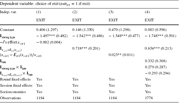
The estimations on effort choices demonstrated the strongest adjustment effect in the EXIT treatment. To understand the role of selection we run logistic random-effects regressions on individual i’s choice
 whether to exit the game at the end of stage 1 of round r.Footnote 34 The estimation results presented in Table 2 confirm a self-selection effect based on the propensity to invest much effort: the probability to exit is significantly lower for strong types (the predicted marginal effect of
 is in the range between
 and
and
 , depending on the exact specification). This biases the sample in stages
 toward strong types so that equilibrium effort should go up as compared to stage 1 (compare Proposition Footnote 5), providing an explanation for Result Footnote 1.
Table 2 Individual choice whether to exit
|
|
||||
|---|---|---|---|---|
|
Indep. var. |
(1) |
(2) |
(3) |
(4) |
|
EXIT |
EXIT |
EXIT |
EXIT |
|
|
Constant |
0.406 (1.297) |
0.146 (1.350) |
0.470 (1.298) |
0.083 (0.596) |
|
|
− 1.497*** (0.482) |
− 1.542*** (0.486) |
− 1.548*** (0.477) |
− 1.748*** (0.501) |
|
|
− 0.002 (0.004) |
|||
|
|
0.718*** (0.201) |
0.654*** (0.213) |
||
|
|
0.023** (0.011) |
|||
|
|
0.332 (0.368) |
|||
|
|
0.279 (0.287) |
|||
|
|
− 0.293 (0.294) |
|||
|
Round fixed effects |
Yes |
Yes |
Yes |
Yes |
|
Session fixed effects |
Yes |
Yes |
Yes |
Yes |
|
Socioeconomics |
Yes |
Yes |
Yes |
Yes |
|
Observations |
1184 |
1184 |
1184 |
1776 |


Random-effects logistic regressions; SE in parentheses, clustered at the level of matching groups; *** (**, *) significant at 1% (5%, 10%). Estimations (1)–(3): data from rounds 6–15; estimation (4): data from rounds 1–15.
 if subject i’s average effort in rounds 1–5 higher than average effort of all subjects in rounds 1–5 of the respective treatment, and
 otherwise.
 if opponent’s actual stage 1 effort > stated beliefs about opponent’s effort, and
 otherwise.
 if round
 and
and
 otherwise
The estimation results in Table 2 also show that the effort of the stage 1 opponent has no significant effect on the probability to exit (compare estimation 1), which is plausible given the random re-matching of player pairs in the subsequent stages. The difference between the stated beliefs
 about the opponent’s effort and the actually observed effort
 , however, can explain the choice to exit: those players who underestimated the opponent’s effort are more likely to exit. This holds when using an indicator variable for whether actual opponent’s effort
 is higher than stated beliefs
 (estimation 2 of Table 2; p value
 ) or when including the (relative) difference of actual effort
 and stated beliefs (estimation 3 of Table 2; p value is 0.028). Even when players are randomly re-matched in later stages, the update in beliefs following the “negative surprise” of unexpectedly high opponent’s effort can make individuals revise their expectations about payoffs to be obtained in later stages and, hence, affect their choice of exit.Footnote 35
Result 3
In the EXIT treatment, weak types are more likely to exit. Moreover, individuals who are negatively surprised by high opponent’s effort in stage 1 are more likely to exit.
Estimation (4) in Table 2 investigates differences in early as compared to late rounds. The self-selection effects measured by the indicator variable for strong types become slightly weaker in later rounds where the subjects have gained some experience but is significant at the
 -level both in early and in late rounds. The effects of beliefs captured by underestimating the opponent’s effort become slightly weaker and less significant in later rounds where updating of beliefs is supposed to be less important.Footnote 36 To summarize, the increase in efforts in later stages of the EXIT treatment is clearly caused by self-selection of strong types into continuing conflict, rather than some kind of misunderstanding and learning of how to play the game. In addition, discouraging signals obtained about the type distribution cause an increase in the probability to exit.
4.4 On beliefs and updating
The theory framework predicts that individual beliefs about the opponent’s effort in early stages/rounds should be positively correlated with the own type (effort), while this correlation is reduced once the individuals have obtained sufficiently many signals about other players’ types through the observed effort choices.Footnote 37 Figure 2 plots the correlation coefficient of own effort and stated beliefs about the respective opponent’s effort over the 15 rounds and the (up to) 5 stages within one round, separately for the sessions with and without monetary incentives for belief elicitation. In both cases, the figure shows a rapid reduction in the correlation in early rounds but then a rather stable positive correlation, suggesting that the own type matters for the beliefs about other players’ types even in later stages/rounds.Footnote 38 While the reduction in correlation is in line with the theory predictions, the persistence of considerable correlation is not explained in our theory. This persistence is, however, well in line with considerable psychological evidence on social projection, the confirmation bias, and in this context on the primacy effect in belief formation (see Marks and Miller Reference Marks and Miller1987 on social projection, and Nickerson Reference Nickerson1998 on the confirmation bias).
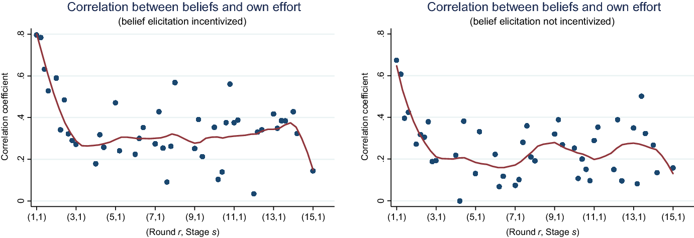
Fig. 2 Correlation between own effort
 and stated beliefs
 about the opponent’s effort (in a given stage and round)
As further evidence on updating of beliefs, Table 4 in Section B.4 of the Online Appendix shows that, similar to the correlation coefficient in Fig. 2, the deviation of stated beliefs from the actual effort of the opponent decreases in the number of signals obtained about others’ efforts (the number of the state contest played) but at a decreasing rate. Put differently, the accuracy of the stated beliefs increases rapidly across the first stages and rounds but the learning effects weaken in later stages where the individuals should already have a rather accurate prior. Again, this holds very similarly for the sessions with and without monetary incentives for the subjects for stating correct beliefs.Footnote 39
Result 4
Individual beliefs about opponents’ efforts are positively correlated with the own type. This correlation is reduced in later stages and rounds.
Within one round, different types of players may adjust their beliefs differently. Table 5 in Section B.6 of the Online Appendix presents random-effects regressions where we estimate the stated beliefs as a function of the stage and distinguish between strong and weak types (we basically use the specifications of Table 1, replacing the dependent variable by individual beliefs
 ). The results confirm the theory predictions in that strong types also hold higher beliefs about the opponent’s effort than weak types. This difference is large in early rounds (26.5 points; compare the coefficient of
 in estimation 2) and becomes smaller in later rounds (estimation 3) where heterogeneity in beliefs is predicted to disappear. Moreover, the adjustment effect of beliefs is more pronounced for strong than for weak types (compare the coefficient of “
 ” in estimations 1–3), in line with theory prediction in the presence of an empirical type distribution exhibiting many weak types where the updating is predicted to be more important for strong than for weak types. More precisely, in early rounds (estimation 2), both types’ beliefs exhibit a large and significant downward adjustment (p values of the coefficients of “
 ” and of the sum of the coefficients of “
 ” and its interaction with

 ), the adjustment being significantly larger for strong types. In later rounds (estimation 3), weak types’ beliefs do not significantly change across stages (see the coefficient of “Stage
 ”; p value is 0.439) and the adjustment of strong types’ beliefs becomes weaker in size and significance (the sum of the coefficients of “
 ” and its interaction with
 is significant at the
 level;
 value is 0.030). Finally, the stage 1 opponent’s effort has a significantly positive effect on the stated beliefs, especially in early rounds and less so in later rounds (see the coefficient of
 in estimations 2 and 3; a similar result is obtained for the previous opponent’s effort
 ). Again, this is in line with the theory mechanism where the individuals update their beliefs from interaction to interaction but at a decreasing rate.
Overall, consistent with the results on individual efforts, the adjustments of beliefs are stronger in early rounds and weakened in late rounds. Also, the difference in average beliefs between strong and weak types is larger in early rounds. Similar adjustment effects in early as compared to late rounds are obtained when estimating strong and weak types’ adjustments of beliefs across contest subgames played. This confirms the importance of the own type for belief formation and updating in early stages and rounds.
5 Conclusions
This paper studied learning and selection and their implications for possible effort escalation in a simple game of dynamic property rights conflict: a multi-stage contest with random resolve. Players who may differ in unobserved preference characteristics encounter changing adversaries in a sequence of contests of stochastic length. They can make use of what they know about their own type and the actions chosen by their previous adversaries. This way they can learn about the underlying population of players and make inference about the types of current and future adversaries. In a corresponding lab experiment, we find that participants exploit the information about their own type (self-projection) and observations about other players’ actions to update their beliefs about future adversaries’ effort. Belief updating can explain type-dependent effort escalation and de-escalation, respectively, across the stages of conflict in an otherwise stationary environment. Moreover, whenever there is a possibility to exit the game, effort escalation is caused by self-selection based on preference heterogeneity and perceptions about the conflict environment. Learning in the experiment falls short of perfectly rational Bayesian updating, however, and psychological behavioral theories of confirmation bias and the primacy effect in belief formation over time seemingly play a role.
The paper contributes both to the theory of conflict and to the methodology of conflict experiments and related strategic interactions. From a methodological perspective, it highlights the role of the theoretical benchmark. The benchmark of equilibrium behavior between identical players who maximize their monetary payoffs under conditions of full information about the environment does not account for problems of incomplete information that the subjects face. Unobserved preference heterogeneity in non-monetary payoff components turns laboratory experiments into games under incomplete information, even when the rules of the game and the structure of monetary payoffs are common knowledge. Consequently, the subjects in the laboratory might suffer from uncertainty about the likely composition of types in the population of players they encounter. Their own types are then predictors about this composition; Bayesian updating causes self-projection in this case. Also, players’ experience from previous interactions provides information about the types that players face in later interactions so that adjustments in behavior across interactions are a natural consequence of standard Bayesian updating. In other words, with type heterogeneity and incomplete information, systematic deviations from the standard theory prediction for symmetric players naturally emerge due to differences in players’ beliefs and experience and, whenever possible, due to self-selection of certain player types. From an ex ante perspective (that is, unconditional on the true type distribution), average behavior under the benchmark of symmetric players or complete information may not be qualitatively very different from the average behavior with uncertainty and updating. But since the adjustments in behavior can depend on a player’s preference type and the distribution of preference types in the population, this is most likely no longer true ex post (that is, conditional on the true type distribution) and at the level of player types. Therefore, the predictions for behavior in a single experiment can be structurally different when taking into account unobserved preference heterogeneity and uncertainty about the true type distribution. Our experiment suggests that these modified predictions can be a suitable benchmark for testing and interpreting conflict behavior.
Welfare considerations are not straightforward and comprise several relevant and conflicting aspects. Contest effort itself can be desirable or wasteful. Much effort might be appreciated in sports competitions, design contests or R&D, and wasteful in military conflict or plain property-rights conflict. In some applications even the welfare assessment of effort is ambiguous. Lobbying effort, for instance, might be informative [as in Skaperdas and Vaidya (Reference Skaperdas and Vaidya2012)], potentially leading to better political decisions, or be simply wasteful [as in the standard Tullock (Reference Tullock and Buchanan1980) approach]. Similarly, a focus on the participants’ payoffs as a measure of welfare leads to ambiguities. We might conclude that an exit option is good for weak players who can enjoy an outside option without fighting a battle against determined fighters. For strong players, an exit option has negative indirect effects at the individual level, as it intensifies the competition between them. But the set of strong players as a whole benefits because exit of weak players allocates the prize among fewer players who value it more. Finally, even though improved information about the population benefits a player when keeping others’ behavior constant, there are countervailing effects on the players’ payoffs due to the different strategic implications of learning for strong and weak players. For instance, learning that the population mostly consists of weak types helps strong players to avoid excessive expenditures but, at the same time, lowers their chances of winning because weak types become more competitive.
One of the main messages of the paper relates to the role of self-projection as a tool for an assessment of potentially unfamiliar conflict situations that involve population uncertainty. If players do not have a sound basis for assessing the types of their adversaries, then self-projection is seemingly a useful device they apply to improve their strategy choices. But in line with evidence from psychology, what they learn from self-projection might be more persistent than what would be optimal. Without going so far as to make recommendations for possible correction policies, the persistence of self-projection and the lack of sufficiently fast updating of prior beliefs may still be useful as a finding when drawing policy conclusions.
Acknowledgements
Open access funding provided by University of Innsbruck and Medical University of Innsbruck.
Appendix 1: proofs of the main theoretical results
Proof of Proposition Footnote 1
Consider the static contest game in the final stage n if n is reached. All actions that were observed in previous stages do not affect beliefs, as
 is common knowledge. This continuation game is equivalent to a static game with incomplete information about
 . Backward induction yields that this is also true for each previous contest encounter. The dynamic problem decomposes into n independent static equilibrium problems, each with the same (but type-dependent) effort choice. All player types expect the opponent’s effort at stage s to be as in (4), based on the commonly known population shares. An interior equilibrium
 is described by the first-order conditionsFootnote 40
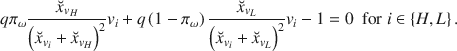
Proof of Proposition Footnote 2
Suppose that stage s is reached (which implies that the prize has not been awarded in any previous stage) and consider the decision problem of player i who is fully characterized by the vector
 . At stage s, a player of type
 forms probability beliefs for all possible types
 . Due to random matching from a set with infinitely many players, these beliefs are also the probability beliefs about the type of the opponent
 at stage s. The player also forms expectations about each type
 ’s effort choice at stage s. Assuming that the effort choices are single-valued we denote these by
 .
.
Denote a player’s expected continuation payoff from stage
 onward by
 . Then, at stage s player i maximizes the objective function
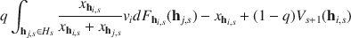
subject to
 . As we will argue further below, the continuation values
 for
for
 are exogenous with respect to a single player’s choice at stage s. We also will show that, for each stage s,
 consists of finite sets of probability atoms in the candidate equilibrium. We use these properties to rewrite the objective function as
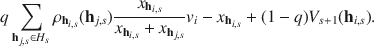
As
 , the objective function is continuous and strictly concave in
 . It must take a unique maximum on the closed and compact support of possible effort choices, and this maximum must be a continuous function of efforts
 . Hence, the optimal choices of the players define a continuous self-mapping
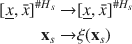
on a convex and compact set, where
 is the number of types in stage s emerging from histories in stages
 to
to
 . Applying Brouwer’s fixed point theorem yields that
 has at least one fixed point, and this fixed point constitutes a vector of equilibrium efforts at stage s. Suppose in what follows that if there are multiple fixed points, the players coordinate on one of them.
Note that
 is comprised of sets with finite numbers of elements on the equilibrium path. For
 , this set has only two elements, as
 . A given set
 with a finite number of types that have positive probabilities that sum up to one leads to a new set of types
 in this equilibrium with the same property: the induced set fulfills all assumptions made about
 , and in particular, is a finite set if
 was a finite set. So, should the contest not resolve at stage s, it moves on to
 and the problem at
 has a larger, but finite number of types and is structurally equivalent to the problem at s.
Also, a player’s belief that
 is independent of a single player’s action at stage s is correct. If a player of type
 deviates from the local equilibrium strategy profile
 at stage s and chooses
 , the deviating behavior is observed by the stage s opponent
 and changes the history type of this player
 . However, given that the contestants are randomly re-matched at each stage and that player
 and all players that
 is matched with constitute a set with zero measure within the set of all players, the deviating behavior does not change the equilibrium composition of types in the next or any other future stage. Therefore, the deviation has no effect on the player’s own payoff in future stages.
Hence, the solution for a perfect Bayesian equilibrium of the game reduces to a series of Bayesian equilibria, one for each possible stage of the game. This sequence of problems is linked only by the fact that the local strategy profile at a given stage together with the equilibrium distribution of types
 at the beginning of stage s jointly determine the equilibrium distribution of types
 at the beginning of stage
 .
.
Proof of Lemma Footnote 1
Ex ante, all players have the same common prior about the likelihood of the two states of the world. With the common prior belief which assigns a probability of 1 / 2 to each of the two states, Bayesian updating leads to
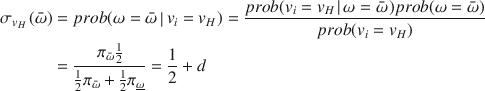
for a player who learns to have a valuation
 . This belief induces a belief about the share of strong types in the population and the probability that the stage 1 opponent is of this type. This share/probability is

Analogously, for a player who learns to have a valuation
 , Bayesian updating yields

so that the posterior belief of weak types about the share of strong types is

We note that
 and
and
 .
.
Proof of Proposition Footnote 3
The stage 1 effort choice of type
 maximizes

Since the continuation payoff
 does not depend on
 , the equilibrium efforts
 in an interior Bayesian Nash equilibrium are the solution of the system of two equations

which are directly obtained from the first-order conditions. Since (23) and (25) imply that
 , combining the two equations in (27) yields

Note that (28) together with
 implies that
 . With (27) and (28) we obtain the equilibrium values (8) and (9). This characterizes the equilibrium effort choices at stage 1 if
 . A sufficient condition for the equilibrium to be interior is that
 and
and
 is sufficiently close to zero.
Each player i anticipates the equilibrium effort levels (8) and (9) of their matched opponent
 , and these anticipated values are independent of i’s own type. But the players’ posterior beliefs about their opponent’s type depend on the own type, as given in (23) and (25). Player i uses this posterior belief to calculate the unconditional expected effort of
 as (10) and (11). Due to
 and
and
 , we get
 .
.
Proof of Proposition Footnote 4
Combining the two first-order conditions (5) and (6) yields the condition
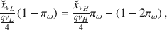
which can be used to establish monotonicity properties of the equilibrium efforts:
 is strictly increasing in
 and
and
 is strictly decreasing in
 .Footnote 41 Moreover,
 and
and
 are continuous is
 , that is, continuous in d, and stage 1 equilibrium efforts
 and
and
 are continuous in d as well. Using (8) and (9),
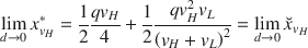
and
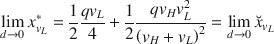
in both states
 .Footnote 42
Part (ii) Suppose that the true share of high-valuation types is
 . Then,
 for all
 . Using (30) and the fact that
 is strictly increasing in
 (Corollary Footnote 1) and
 is strictly increasing in
 , it follows that
 for all
 . Note that
 is lowest if
 in which case
 converges to
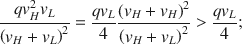
hence, for all
 ,
,
 is higher than the stage 1 effort
 of weak types (which is at most
 , in case
 ).
).
Now consider the low-valuation types. With the first-order condition for
 ,
,

Here, the first inequality follows from
 ; the second inequality follows from
 .Footnote 43 Let
 and suppose that
 . Then, the right-hand side of inequality (33) is (weakly) smaller than
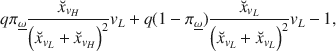
which is equal to zero by (18); contradiction. Therefore, we must have
 . If
. If
 , the probability that weak types attach to facing another weak type converges to one so that both
 and
and
 converge to
 .
.
Part (i) Suppose that the true share of high-valuation types is
 . Then,
 for all
 . Using (31) and the fact that
 is strictly increasing in
 (Corollary Footnote 1) and
 is strictly increasing in
 , it holds that
 .
.
Note that the proof of Proposition Footnote 4 only makes use of the rankings
 as well as
 and
and
 , but does not use, for instance, that
 and
and
 for the assumed information structure. In other words, the result in Proposition Footnote 4 does not qualitatively depend on the players knowing the exact share of high and low players in the population. It is sufficient that the players hold common beliefs about the type distribution and that the beliefs about the share of high types are corrected upward in case of
 , and are corrected downward in case of
 .
.
In contrast, in case of
 , comparisons of
 to
to
 rely on the difference between
 and
and
 . It is possible (although more complex) to show that
 for all
 with
with
 if d is sufficiently small. However,
 may be smaller than
 if d is very close to 1 / 2 and
 is large compared to
 .Footnote 44
Proof of Proposition Footnote 5
Suppose all players i with
 exit and all players j with
 continue in stage 2. We have to show that no single player has an incentive to deviate from the candidate equilibrium behavior. In the candidate equilibrium, the players anticipate that the common beliefs among all players is that (almost) all players who remain active in stage 2 have
 . Hence, players with
 choose an equilibrium effort of
 in all stages
 and earn an expected payoff from staying active of
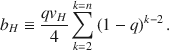
A player i with valuation
 can also anticipate that
 for all
 and chooses her effort
 as the best reply. Straightforward calculus yields this best reply as
 with
with
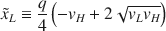
at all stages
 . Denote the resulting continuation value for weak types by

Hence, it is optimal for weak types to exit and for strong types to stay if
 .
.
Note that the interval
 is non-empty. If
 then
then
 simplifies to

which is strictly smaller than
 given above. If instead
 then
then
 is equal to

where the second inequality holds whenever strong types strictly prefer an effort
 over an effort
 .
.


 xirs
xirs Eirsx-irs


 Open access