


1 Introduction
This Element is about agent-based macroeconomics in general, and in particular about a family of evolutionary Agent-Based Models (ABMs), which we call ‘Schumpeter meeting Keynes’ (or K+S). There are four fundamental features of the K+S family of agent-based models. The first is the complementarity between a Schumpeterian engine of innovation and a Keynesian engine of demand generation. Second, the models entail the intrinsic duality of wages, which are an item of cost for individual firms but also a component of aggregate demand. Third, there is a permanent duality between the labour-shedding effects of technical change via productivity improvements and its employment generation via the introduction of new products. Finally, fourth, ubiquitous institutions shape the rules of behaviours of individual agents and their pattern of interaction. As with all well-constructed ABMs, the K+S models are populated by a multiplicity of agents which interact on the grounds of quite simple, empirically based, behavioural rules, whose collective outcomes are ‘emergent properties’ which cannot be imputed to the intention of any single agent.
All this modelling perspective would sound quite straightforward were it not for the dismal state of current macroeconomics. Thus, given the latter, it might be appropriate to start by arguing why we need a ‘macro’ level of analysis well nested into valid microfoundations in the first place, which is perfectly obvious in all other natural and social disciplines, but not in economics. Next we shall place our presentation of ABMs against the background of the vicissitudes of modern macroeconomics as prolegomena to the core of this Element, the K+S family of macro ABMs.
With the noticeable exception of a good deal of contemporary economics, almost all scientific disciplines, both natural and social ones, distinguish between ‘lower’, more micro, levels of description of whatever phenomenon, and ‘high-level’ ones, regarding collective outcomes, which are typically not isomorphic to the former.Footnote 1 So, in physics, thermodynamics is not postulated on the kinetic properties of some ‘representative’ or ‘average’ molecules! And even more so in biology, ethology, or medicine. This is a fundamental point repeatedly emphasised by Kirman (Reference Kirman2016) and outside our discipline by Anderson (Reference Anderson1972) and Prigogine (Reference Prigogine1980), among a few outstanding others. The basic epistemological notion is that the aggregate of interacting entities yields emergent properties, which cannot be mapped down to the (conscious or unconscious) behaviours of some identifiable underlying components.Footnote 2 This is so obvious to natural scientists that it would be an insult to them to remind them that the dynamics of a beehive cannot be summarised by the dynamic adjustment of a ‘representative bee’ (the example is discussed, again, in Kirman, Reference Kirman2016). The relation between ‘micro’ and ‘macro’ has been at the very centre of all social sciences since their inception. Think of one of the everlasting questions, namely the relationship between agency and structure, which is at the core of most interpretations of social phenomena. Or, nearer to our concerns here, consider the (often misunderstood) notion of Adam Smith’s invisible hand: this is basically a proposition about the lack of isomorphisms between the greediness of individual butchers and bakers, on the one hand, and the relatively orderly delivery of meat and bread across markets.
Unfortunately, what is obvious for the scientific community is unknown or ignored by current macroeconomics. Indeed, after a fruitful infancy in which the early Keynesian macroeconomic theories focused on the laws of motion of capitalist dynamics, also embedding some notions of disequilibrium and coordination failures, the discipline in the 1970s took a perverse path, relying on models grounded on fictitious rational representative agents in a pathetic attempt to circumvent aggregation and coordination problems. Such fraudulent microfoundations shrink the macro level to the optimising behaviour of one agent, thus losing all the complex dynamics emerging when one moves to the higher levels. The Dark Age of macroeconomics reached the abyss with the Great Recession of 2008, the biggest downturn that had hit developed economies since 1929. Not only was representative-agent macroeconomic theory unable to explain what happened in 2008, but it was instrumental to the crisis. Indeed, if macroeconomic models are grounded on a lonely agent, how could one study the rising of income inequality and financialisation which paved the way to the subprime mortgage crisis? A new macroeconomics paradigm is thus urgently needed.
In the new alternative paradigm, which inspires this Element, macroeconomics should consider the economy as a complex, evolving system, an ecology populated by heterogeneous agents (e.g. firms, workers, banks) whose far-from-equilibrium local interactions yield some collective order, even if the structure of the system continuously changes (more on that in Farmer & Foley, Reference Farmer and Foley2009; Kirman, Reference Kirman2010b, Reference Kirman2016; Rosser, Reference Rosser2011; Dosi, Reference Dosi2014, Reference Dosi2023; Dosi & Virgillito, Reference Dosi and Virgillito2017; Dosi & Roventini, Reference Dosi and Roventini2019). In such a framework, first, more is different (Anderson, Reference Anderson1972): to repeat, there is not any isomorphism between the micro- and macroeconomic levels, and higher levels of aggregation can lead to the emergence of new phenomena (e.g. business cycles and self-sustained growth), new statistical regularities (e.g. Kaldor–Verdoorn and Okun’s laws), and completely new structures (i.e. new firms, new industries, new markets, and new institutions).
Second, the economic system exhibits self-organised criticality: imbalances can build over time, leading to the emergence of tipping points which can be triggered by apparently innocuous shocks. (This is straightforward in climate change, see Steffen et al., Reference Steffen, Rockström, Richardson, Folke, Liverman, Summerhayes, Barnosky, Cornell, Crucifix, Donges, Fetzer, Lade, Scheffer, Winkelmann and Schellnhuber2018; but with regard to other fields in economics, see Bak et al., Reference Bak, Chen, Scheinkman and Woodford1992 and Battiston et al., Reference Battiston, Farmer and Flache2016.)
Third, in a complex world, deep uncertainty (Keynes, Reference Keynes1921, Reference Keynes1936; Knight, Reference Knight1921; Dosi, Reference Dosi2023) is so pervasive that agents cannot build the ‘right’ model of the economy, and, even less so, share it among them as well as with the modeller (Kirman, Reference Kirman2014).
Fourth, behaviours typically rely on heuristics (Simon, Reference Simon1955, Reference Simon1959; Cyert & March,Reference Cyert and March1992; Dosi, Reference Dosi2023), which turns out to be a robust set of tools for inference and actions (Gigerenzer & Brighton, Reference Gigerenzer and Brighton2009; Haldane, Reference Haldane2012; Dosi et al., Reference Dosi, Napoletano, Roventini, Stiglitz and Treibich2020a).
Of course, fifth, local interactions among purposeful agents cannot be generally assumed to lead to efficient outcomes or optimal equilibria.
Finally, from a normative point of view, when complexity is involved, policy makers ought to aim at resilient systems which often require redundancy and degeneracy (Edelman & Gally, Reference Edelman and Gally2001). To put it in a provocative way: would someone fly on a plane designed by a team of New Classical macroeconomists, who sound much like the early aerodynamic scholars who conclusively argued that, in equilibrium, airplanes cannot fly?
Once complexity is seriously taken into account in macroeconomics, one, of course, has to rule out Dynamic Stochastic General Equilibrium (DSGE) models. A natural alternative candidate, we shall argue, is Agent-Based Computational Economics (ACE; Tesfatsion, Reference Tesfatsion, Tesfatsion and Judd2006; LeBaron & Tesfatsion, Reference LeBaron and Tesfatsion2008; Fagiolo & Roventini, Reference Fagiolo and Roventini2017; Caverzasi & Russo, Reference Dawid, Delli Gatti, Hommes and LeBaron2018; Dawid & Delli Gatti, Reference Caverzasi and Russo2018), which straightforwardly embeds heterogeneity, bounded rationality, endogenous out-of-equilibrium dynamics, and direct interactions among economic agents. In so doing, ACE provides an alternative way to build macroeconomic models with genuine microfoundations, which take seriously the problem of aggregation and are able to jointly account for the emergence of self-sustained growth and business cycles punctuated by major crises. Furthermore, on the normative side, due to the flexibility of their set of assumptions regarding agent behaviours and interactions, ACE models represent an exceptional laboratory to design policies and to test their effects on macroeconomic dynamics.
As recalled by Haldane and Turrell (Reference Haldane and Turrell2019), the first prototypes of agent-based models were developed by Enrico Fermi in the 1930s in order to study the movement of neutrons. (Of course, Fermi, a Nobel laureate physicist, never thought to build a model sporting a representative neutron!) With adoption of Monte Carlo methods, ABMs flourished in many disciplines, ranging from physics, biology, ecology, epidemiology, all the way to the military (more on that in Turrell, Reference Turrell2016). Recent years have also seen a surge of agent-based models in macroeconomics (see Fagiolo & Roventini, Reference Fagiolo and Roventini2012, Reference Fagiolo and Roventini2017 and Dawid & Delli Gatti, Reference Dawid, Delli Gatti, Hommes and LeBaron2018 for surveys): an increasing number of papers involving macroeconomic ABMs have also addressed the policy domain concerning, for example, fiscal policy, monetary policy, macroprudential policy, labour market policy, and climate-change policy. And ABMs have been increasingly part of the policy tools in, for example, central banks and other institutions in ways complementary to older macroeconomic models (Haldane & Turrell, Reference Haldane and Turrell2019).Footnote 3
The rest of the Element is organised as follows. In Section 2, we will provide a short story of macroeconomics focusing on the problem of aggregation and, more generally, on its relationship with microeconomics. Section 3 discusses the insurmountable limits of neoclassical macroeconomics, focusing on its latest incarnation, the DSGE models. In Section 4 we introduce agent-based macroeconomics, and in Section 5 we present the family of Keynes meeting Schumpeter agent-based models. The empirical validation of the K+S models is performed in Section 6, while the impacts of different combinations of innovation, industrial, fiscal, and monetary policies for different labour-market regimes and inequality scenarios are assessed in Section 7. Finally, in Section 8 we conclude with a brief discussion on the future of macroeconomics.
2 A Dismal Short Story of Macroeconomics: From Robinson Crusoe to Complex Evolutionary Economies
The relationship between the micro and the macro is at the core of the (lack of) evolution of macroeconomics and it has a fundamental role in explaining why the 2008 financial crisis was also a crisis for macroeconomic theory (Kirman, Reference Kirman2010b). Indeed, standard DSGE models not only failed to forecast the crisis, but they did not even admit the possibility of such an event, leaving policy makers without policy solutions (Krugman, Reference Krugman2011). In this section, we briefly outline the path that macroeconomics has been following for the last ninety years (Sections 2.1–2.4).Footnote 4 Together, we will shed light on the dismal status of the discipline, which appears incapable of explaining the phenomena – that is, crises and depressions – for which it was born (see Section 2.5).
2.1 The Happy Childhood of Macroeconomics
Roughly speaking, macroeconomics first saw the light of day with Keynes. For sure, enlightening analyses came before, including Wicksell’s, but the distinctiveness of macro levels of interpretation came with him. Indeed, up to the 1970s, there were basically two ‘macros’.
One was equilibrium growth theories. While it is the case that, for example, models á la Solow invoked maximising behaviours in order to establish equilibrium input intensities, no claim was made that such allocations were the work of any ‘representative agent’ in turn taken to be the ‘synthetic’ (??) version of some underlying General Equilibrium (GE). By the same token, the distinction between positive (that is, purportedly descriptive) and normative models, before Lucas and his companions, was absolutely clear to the practitioners. Hence, the prescriptive side was kept distinctly separated. Ramsey (Reference Ramsey1928) – type models, asking what a benevolent central planner would do, were reasonably kept apart from any question on the ‘laws of motion’ of capitalism, á la Harrod (Reference Harrod1939), Domar (Reference Domar1946), Kaldor (Reference Kaldor1957), and indeed Solow (Reference Solow1956). Finally, in the good and in the bad, technological change was kept separate from the mechanisms of resource allocation: the famous ‘Solow residual’ was, as is well known, the statistical counterpart of the drift in growth models with an exogenous technological change.
Second, in some fuzzy land between purported GE ‘microfoundations’ and equilibrium growth theories, lived for at least three decades a macroeconomics sufficiently ‘Keynesian’ in spirit and quite neoclassical in terms of tools. It was the early ‘neo-Keynesianism’ (also known as the Neoclassical Synthesis) – pioneered by Hicks (Reference Hicks1937), and shortly thereafter by Modigliani, Samuelson, Patinkin, and a few other American ‘Keynesians’ – whom Joan Robinson contemptuously defined as ‘bastard Keynesians’. It is the short-term macro which students used to learn up to the 1980s, with IS-LM curves, which are meant to capture the aggregate relations between money supply and money demand, interest rates, savings, and investments; Phillips curves on the labour market; and a few other curves as well. In fact, the curves were (are) a precarious compromise between the notion that the economy is supposed to be in some sort of equilibrium – albeit of a short-term nature – and the notion of a more ‘fundamental’ equilibrium path to which the economy is bound to tend in the longer run.
That was a kind of mainstream, especially on the other side of the Atlantic. There was also a group of thinkers whom we could call (as they called themselves) genuine Keynesians. They were predominantly in Europe, especially in the UK and in Italy: see Pasinetti (Reference Pasinetti1974), (Reference Pasinetti1983) and Harcourt (Reference Harcourt2007) for an overview.Footnote 5 The focus was only on the basic laws of motions of capitalist dynamics. They include the drivers of aggregate demand; the multiplier leading from the ‘autonomous’ components of demand such as government expenditures and exports to aggregate income; the accelerator, linking aggregate investment to past variations in aggregate income itself; and the relation between unemployment, wage/profits shares, and investments.Footnote 6 Indeed, such a stream of research is alive and progressing, refining upon the modelling of the ‘laws of motion’ and their supporting empirical evidence: see Lavoie (Reference Lavoie2009); Lavoie and Stockhammer (Reference Lavoie and Stockhammer2013); and Storm and Naastepad (Reference Storm and Naastepad2012a, Reference Storm and Naastepad2012b), among quite a few others.
Indeed, a common characteristic of the variegated contributions from ‘genuine Keynesianism’, often known also as post-Keynesian, is the scepticism about any microfoundation, to its own merit and also to its own peril. Part of the denial comes from a healthy rejection of methodological individualism and its axiomatisation as the ultimate primitive of economic analysis. Part of it, in our view, comes from the misleading notion that microfoundations necessarily mean methodological individualism (as if the interpretation of the working of a beehive had to necessarily build upon the knowledge of ‘what individual bees think and do’, or indeed ‘should do’). On the contrary, microfoundations might well mean how the macro structure of the beehive influences the distribution of the behaviours of the bees, a sort of macrofoundation of the micro. All this entails a major terrain of dialogue between the foregoing stream of Keynesian models and agent-based ones.
Now, back to the roots of modern macroeconomics. The opposite extreme to ‘bastard Keynesianism’ was not Keynesian at all, even if it sometimes took up the IS-LM-Phillips discourse. The best concise synthesis is Friedman (Reference Friedman1968). Historically it went under the heading of monetarism, but basically it was the pre-Keynesian view that the economy left to itself travels on a unique equilibrium path in the long- and short-run. Indeed, in a barter, pre-industrial economy where Say’s law and the quantitative theory of money hold, monetary policy cannot influence the interest rate and fiscal policy completely crowds out private consumption and investment: ‘there is a natural rate of unemployment which policies cannot influence’; see the deep discussion in Solow (Reference Solow2018). Milton Friedman was the obvious ancestor of Lucas and his companions, but he was still too far from the subsequent axioms, awaiting any empirical proof of plausibility.Footnote 7
2.2 ‘New Classical (??)’ Talibanism and Beyond
What happened next? Starting from the beginning of the 1970s, we think that everything which could get worse got worse and more: accordingly, we agree with Krugman (Reference Krugman2011) and Romer (Reference Romer2016) that macroeconomics plunged into a Dark Age.Footnote 8
First, ‘new classical economics’ (even if the reference to the Classics could not be further far away) fully abolished the distinction between the normative and positive domains – between models á la Ramsey and models á la Harrod-Domar, Solow, and so on (notwithstanding the differences amongst the latter ones). In fact, the striking paradox for theorists who are in good part market talibans is that they start with a model which is essentially of a benign, forward-looking, central planner, and only at the end, by way of an abundant dose of hand-waving, claim that the solution of whatever intertemporal optimisation problem is in fact supported by a decentralised market equilibrium.
Things could be much easier for this approach if one could build a genuine ‘general equilibrium’ model (that is, with many agents, heterogeneous at least in their endowments and preferences). However, this is not possible for the well-known, but ignored Sonnenschein (Reference Sonnenschein1972), Mantel (Reference Mantel1974), and Debreu (Reference Debreu1974) theorems (more in Kirman, Reference Kirman1989). Assuming by construction that the coordination problem is solved by resorting to the ‘representative agent’ fiction is simply a pathetic shortcut which does not have any theoretical legitimacy (Kirman, Reference Kirman1992).
Anyhow, the ‘New Classical’ restoration went so far as to wash away the distinction between ‘long-term’ and ‘short-term’ – with the latter as the locus where all ‘frictions’, ‘liquidity traps’, Phillips curves, some (temporary!) real effects of fiscal and monetary policies, and so on had precariously survived before. Why would a representative agent endowed with ‘rational’ expectations able to solve sophisticated inter-temporal optimization problems from here to infinity display any friction or distortion in the short-run, if competitive markets always clear? We all know the outrageously silly propositions, sold as major discoveries, also associated with an infamous ‘rational expectation revolution’ concerning the ineffectiveness of fiscal and monetary policies and the general properties of markets to yield Pareto first-best allocations. (In this respect, of course, it is easier for that to happen if ‘the market’ is one representative agent: coordination and allocation failures would involve serious episodes of schizophrenia by that agent itself!).
While Lucas and Sargent Reference Lucas and Sargent1978 wrote an obituary of Keynesian macroeconomics, we think that in other times, nearly the entire profession would have reacted to such a ‘revolution’ as Bob Solow once did when asked by Klamer (Reference Klamer1984) why he did not take the ‘new Classics’ seriously:
Suppose someone sits down where you are sitting right now and announces to me he is Napoleon Bonaparte. The last thing I want to do with him is to get involved in a technical discussion of cavalry tactics at the battle of Austerlitz. If I do that, I am tacitly drawn in the game that he is Napoleon. Now, Bob Lucas and Tom Sargent like nothing better than to get drawn in technical discussions, because then you have tacitly gone along with their fundamental assumptions; your attention is attracted away from the basic weakness of the whole story. Since I find that fundamental framework ludicrous, I respond by treating it as ludicrous — that is, by laughing at it — so as not to fall in the trap of taking it seriously and passing on matters of technique.
The reasons why the profession, and even worse, the world at large took these ‘Napoleons’ seriously, we think, have basically to do with a Zeitgeist where the hegemonic politics was that epitomized by Ronald Reagan and Margaret Thatcher, and their system of beliefs on the ‘magic of the market place’, ‘society does not exist, only individuals do’, et similia. And, tragically, this set of beliefs became largely politically bipartisan, leading to financial deregulation, massive waves of privatisation, tax cuts and surging inequality, and so on. Or think of the disasters produced for decades around the world by the IMF-inspired Washington Consensus or by the latest waves of austerity and structural-reform policies in the European Union as another such creed on the magic of markets, the evil of governments, and the miraculous effects of blood, sweat, and tears (Fitoussi & Saraceno, Reference Fitoussi and Saraceno2013, refers to this as the Berlin–Washington consensus). The point we want to make is that the changes in the hegemonic (macro) theory should be primarily interpreted in terms of the political economy of power relations among social and political groups, with little to write home about ‘advancements’ in the theory itself ... On the contrary!
The Mariana Trench of fanaticism was reached with Real Business Cycle (RBC) models (Kydland & Prescott, Reference Kydland and Prescott1982) positing optimal Pareto business cycles driven by economywide technological shocks [sic]. The natural question immediately arising concerns the nature of such shocks. What are they? Are recessions driven by episodes of technological regress (e.g. people going back to wash clothes in rivers or suddenly using candles for lighting)? The candid answer provided by one of the founding fathers of RBC theory is that: ‘They’re that traffic out there’ (‘there’ refers to a congested bridge, meaning some mysterious crippling of the ‘invisible hand’, as cited in Romer, Reference Romer2016: p. 5). Needless to say, the RBC propositions were (and are) not supported by any empirical evidence. But the price paid by macroeconomics for this sort of intellectual trolling was and still is huge!
2.3 New Keynesians, New Monetarists and the New Neoclassical Synthesis
Since the 1980s, ‘New Keynesian’ economists, instead of following Solow’s advices,Footnote 9 basically accepted the New Classical and RBC framework and worked on the edges of auxiliary assumptions. So, they introduced monopolistic competition and a plethora of nominal and real rigidities into models with representative-agent cum rational-expectations microfoundations. New Keynesian models restored some basic results which were undisputed before the New Classical Middle Ages, such as the non-neutrality of money. However, the price paid to talk just to ‘New Classicals’ and RBC talibans was tall. The methodological infection was so deep that Mankiw and Romer (Reference Mankiw and Romer1991) claimed that New Keynesian macroeconomics should be renamed New Monetarist macroeconomics, and De Long (Reference De Long2000) discussed ‘the triumph of monetarism’. ‘New Keynesianism’ of different vintages represents what we could call homeopathic Keynesianism: the minimum quantities to be added to the standard model, sufficient to mitigate the most outrageous claims of the latter.
Indeed, the widespread sepsis came with the appearance of a New Neoclassical Synthesis (NNS) (Goodfriend, Reference Goodfriend2007), grounded upon DSGE models (Clarida, Galí, & Gertler, Reference Clarida, Galí and Gertler1999; Woodford, Reference Woodford2003; Galí & Gertler, Reference Galí and Gertler2007). In a nutshell, such models have a RBC core supplemented with monopolistic competition, nominal imperfections, and a monetary policy rule, and they can accomodate various forms of ‘imperfections’, ‘frictions’, and ‘inertias’. To many respects DSGE models are simply the late-Ptolemaic phase of the theory: add epicycles at full steam without any theoretical and empirical discipline in order to better match a particular set of the data. Of course, in the epicycles frenzy one is never touched by a sense of the ridiculous in assuming that the mythical representative agent at the same time is extremely sophisticated when thinking about future allocations, but falls into backward-looking habits when deciding about consumption or, when having to change prices, is tangled by sticky prices! (Caballero, Reference Caballero2010: offers a thorough picture of this surreal state of affairs.) Again, Bob Solow gets straight to the point:Footnote 10
But I found the advent of – Dynamic Stochastic General Equilibrium models to be, not so much as a step backwards, but as a step out of economics. In fact, I’ve been criticized, probably justly, for making jokes about it, but it struck me as funny, as not something you could take seriously. There were times when you start reading an article in that vein, and it would start by saying, “Well, we are going to write down a micro-founded model.” It meant an economy with one person in it, and organized so that the economy carried out the wishes of that person. Well, when I was growing up and getting interested in economics, the essence of economics was that there were people and groups of people in the economy who had conflicting interests. Not only did they want different things, opposing things, they believed different things. And there’s no place for that in what passes, or what was passing a dozen years ago, for a micro-founded model.
Not all New Keynesian economists deliberately choose to step out of economics. Indeed, ‘New Keynesianism’ is a misnomer, in that sometimes it is meant to cover also simple but quite powerful models whereby Keynesian system properties are obtained out of otherwise standard microfoundations, just taking seriously ‘imperfections’ as structural, long-term characteristics of the economy. Pervasive asymmetric information requires some genuine heterogeneity and interactions among agents (see Akerlof & Yellen, Reference Akerlof and Yellen1985; Greenwald & Stiglitz, Reference Greenwald and Stiglitz1993a, Reference Greenwald and Stiglitz1993b; Akerlof, Reference Akerlof2002, Reference Akerlof2007, among others) yielding Keynesian properties as ubiquitous outcomes of coordination failures (for more detailed discussions of Stiglitz’s contributions, see Dosi & Virgillito, Reference Dosi and Virgillito2017).Footnote 11 All that, still without considering the long-term changes in the so-called fundamentals, technical progress, and so on.
2.4 What about Innovation Dynamics and Long-Run Economic Growth?
We have argued that even the coordination issue has been written out of the agenda by assuming it as basically solved by construction. But what about change? What about the ‘Unbound Prometheus’ (Landes, Reference Landes1969) of capitalist search, discovery, and indeed destruction?
In Solow (Reference Solow1956) and subsequent contributions, technical progress appears by default, but it does so in a powerful way as the fundamental driver of long-run growth, to be explained outside the sheer allocation mechanism.Footnote 12 On the contrary, in the DSGE workhorse, there is no Prometheus: ‘innovations’ come as exogenous technology shocks upon the aggregate production function, with the same mythical agent optimally adjusting its consumption and investment plans. And the macroeconomic time series generated by the models are usually de-trended to focus on their business cycle dynamics.Footnote 13 End of the story.
The last thirty years have seen also the emergence of new growth theories (see e.g. Romer, Reference Romer1990; Aghion & Howitt, Reference Aghion and Howitt1992), bringing – as compared to the original Solow model – some significant advancements and, in our view, equally significant drawbacks. The big plus is the endogenisation of technological change: innovation is endogenised into economic dynamics. But that is done just as either a learning externality or as the outcome of purposeful expensive efforts by profit-maximising agents. In the latter case, the endogenisation comes at what we consider the major price (although many colleagues would deem it as a major achievement) of reducing innovative activities to an equilibrium outcome of optimal intertemporal allocation of resources, with or without (probabilisable) uncertainty. Hence, by doing that, one loses also the genuine Schumpeterian notion of innovation as a disequilibrium phenomenon (at least as a transient!).
Moreover, ‘endogenous growth’ theories do not account for business cycles’ fluctuations. This is really unfortunate, as Bob Solow (Reference Solow2005) puts it:
Neoclassical growth theory is about the evolution of potential output. In other words, the model takes it for granted that aggregate output is limited on the supply side, not by shortages (or excesses) of effective demand. Short-run macroeconomics, on the other hand, is mostly about the gap between potential and actual output. ... Some sort of endogenous knitting-together of the fluctuations and growth contexts is needed, and not only for the sake of neatness: the short run and its uncertainties affect the long run through the volume of investment and research expenditure, for instance, and the growth forces in the economy probably influence the frequency and amplitude of short-run fluctuations. ... To put it differently, it would be a good thing if there were a unified macroeconomics capable of dealing with trend and fluctuations, rather than a short-run branch and a long-run branch operating under quite different rules. My quarrel with the real business cycle and related schools is not about that; it is about whether they have chosen an utterly implausible unifying device.
And the separation between growth and business cycle theories is even more problematic given the bourgeoning new empirical literature on hysteresis (among many others, see Dosi et al., Reference Dosi, Pereira, Roventini and Virgillito2018a; Cerra, Fatás, & Saxena Reference Cerra, Fatás and Saxena2023, and the literature cited therein), which convincingly shows the existence of many interlinkages between short-run and long-run phenomena. In particular, in the presence of hysteresis, recessions can permanently depress output, thus undermining the very growing capabilities of economies. On the policy side, this calls for a more active role of fiscal and monetary interventions during downturns, and, more generally, to consider the impact of policies across the whole spectrum of frequencies. On the theoretical side, hysteresis is not due to market imperfections, but rather to the very functioning of decentralised economies characterised by coordination externalities and dynamic increasing returns. In that respect, this Element shows that evolutionary agent-based models are genuinely able to account for the emergence of hysteresis, while providing a unified analysis of technological change and long-run growth together with coordination failures and business cycles.
2.5 From the ‘Great Moderation’ to the Great Recession
In the beginning of this century, under the new consensus reached by the New Neoclassical Synthesis (NNS), Robert E. Lucas, Jr, (Reference Lucas2003) without any embarrassment, declared ‘The central problem of depression prevention had been solved’, and Prescott religiously believed that: ‘This is the golden age of macroeconomics’.Footnote 14 Moreover, a large number of NNS contributions claimed that economic policy was finally becoming more of a science (!?), (Galí & Gertler, Reference Galí and Gertler2007; Goodfriend, Reference Goodfriend2007; Mishkin, Reference Mishkin2007; Taylor, Reference Taylor2007).Footnote 15 This was made possible by the ubiquitous presence of DSGE models in academia and a universe of politicians and opinion-makers under the ‘free market’ / ‘free Wall Street’ globalization spell,Footnote 16 and helped by the ‘divine coincidence’, whereby inflation targeting, performed under some form of Taylor rule, appeared to be a sufficient condition for stabilising the whole economy. During this Panglossian period, some economists went as far as claiming that the ‘scientific approach’ to macroeconomics policy incarnated in DSGE models was the ultimate cause of the so-called Great Moderation (Bernanke, Reference Bernanke2004), namely the fall of GDP volatility experienced by most developed economists since the beginning of the 1980s, and that only minor refinements to the consensus workhorse model were needed.
Unfortunately, as happened with the famous statement made by Francis Fukuyama (Reference Fukuyama1992) about an alleged ‘end of history’,Footnote 17 these positions have been proven to be substantially wrong by subsequent events. Indeed, a relatively small ‘micro’ event, the bankruptcy of Lehman Brothers in 2008, triggered a major financial crisis which caused the Great Recession, the deepest downturn experienced by developed economies since 1929.
In that respect, the Great Recession turned out to be a ‘natural experiment’ for economic analysis, showing the inadequacy of the predominant theoretical frameworks. Indeed, as Krugman (Reference Krugman2011) points out, not only did DSGE models not forecast the crisis, but they did not even admit the possibility of such an event and, even worse, they did not provide any useful advice to policymakers on how to put the economy back on a steady growth path (see also Turner, Reference Turner2010; Stiglitz, Reference Stiglitz2011, Reference Stiglitz2015; Bookstaber, Reference Bookstaber2017; Caverzasi & Russo, Reference Caverzasi and Russo2018; Haldane & Turrell, Reference Haldane and Turrell2019).
Scholars of DSGE have reacted to such a failure by trying to amend their models with a new legion of epicycles; for example, financial frictions, homeopathic doses of agent heterogeneity, bounded rationality, and exogenous fat-tailed shocks (see e.g. Lindé, Smets, & Wouters, Reference Lindé, Wouters, Taylor and Uhlig2016, and the discussion in Section 3.4). Conversely, an increasing number of economists have claimed that the 2008 ‘economic crisis is a crisis for economic theory’ (Colander et al., Reference Colander, Folmer and Haas2009; Farmer & Foley, Reference Farmer and Foley2009; Krugman, Reference Krugman2009, Reference Krugman2011; Caballero, Reference Caballero2010; Kirman, Reference Kirman2010b, Reference Kirman2016; Kay, Reference Kay2011; Stiglitz, Reference Stiglitz2011, Reference Stiglitz2015; Dosi, Reference Dosi2014; Romer, Reference Romer2016; Stiglitz, Reference Stiglitz2017). Indeed, history is the smoking gun against the deeply flawed basic assumptions of mainstream DSGE macroeconomics, for example rational expectations and representative agents, which prevents, by construction, the understanding of the emergence of deep downturns together with standard fluctuations (Stiglitz, Reference Stiglitz2015) and, more generally, the very dynamics of economies. Indeed, resorting to representative-agent microfoundations, how can one understand central phenomena such as rising inequality, bankruptcy cascades and systemic risks, innovation, structural change, and their co-evolution with climate dynamics?
3 The Emperor Is Still Naked: The Intrinsic Limits of DSGE Models
In line with the RBC tradition, the backbone of DSGE models (Clarida et al., Reference Clarida, Galí and Gertler1999; Woodford, Reference Woodford2003; Galí & Gertler, Reference Galí and Gertler2007) is a standard stochastic equilibrium model with variable labour supply: the economy is populated by an infinitely everlasting representative household, and by a representative firm, whose homogenous production technology is hit by exogenous shocks.Footnote 18 All agents form their expectations rationally (Muth, Reference Muth1961). The New Keynesian flavor of the model is provided by money, monopolistic competition, and sticky prices. Money has usually only the function of unit of account, and the nominal rigidities incarnated in sticky prices allow monetary policy to affect real variables in the short run. The RBC scaffold of the model allows the computation of the ‘natural’ level of output and real interest rate, that is, the equilibrium values of the two variables under perfectly flexible prices. In line with the Wickselian tradition, the ‘natural’ output and interest rate constitute a benchmark for monetary policy: the central bank cannot persistently push the output and the interest rate away from their ‘natural’ values without creating inflation or deflation. Finally, imperfect competition and possibly other real rigidity imply that the ‘natural’ level of output might not be socially efficient.
Dynamic Stochastic General Equilibrium models are commonly represented by means of vector auto-regression (VAR) models usually estimated by employing full-information Bayesian techniques (see e.g. Smets & Wouters, Reference Smets and Wouters2003, Reference Smets and Wouters2007). Different types of shocks are usually added to improve the estimation. Moreover, as the assumption of forward-looking agents prevents DSGE models from matching the econometric evidence on the co-movements of nominal and real variables (e.g., the response of output and inflation to a monetary policy shock is too fast to match the gradual adjustment showed by the corresponding empirical impulse-response functions), a legion of ‘frictions’ – generally not justified on theoretical grounds – is introduced, such as predetermined price and spending decisions, indexation of prices and wages to past inflation, sticky wages, habit formation in preferences for consumption, adjustment costs in investment, variable capital utilization, among others. Once the parameters of the model are estimated and the structural shocks are identified, policy-analysis exercises are carried out assuming that the DSGE model is the ‘true’ data-generating process of the available time series.
The usefulness of DSGE models is undermined by plenty of theoretical, empirical, and political-economy problems. Let us discuss each of them in turn (see Fagiolo & Roventini, Reference Fagiolo and Roventini2017: for a more detailed analysis).
3.1 Theoretical Issues
As already mentioned previously, DSGE models suffer the same well-known problems as Arrow–Debreu general-equilibrium models (see Kirman, Reference Kirman1989: for a classical reference) and more. Neglecting them does not mean solving them. On the contrary!
More specifically, the well-known Sonnenschein (Reference Sonnenschein1972), Mantel (Reference Mantel1974), and Debreu (Reference Debreu1974) theorems show that neither the uniqueness nor, and even less so, the stability of the general equilibrium can be attained, even if one employs stringent and unrealistic assumptions about agents, even under amazing information requirements. Indeed, Saari and Simon (Reference Saari and Simon1978) show that an infinite amount of information is required to reach the equilibrium for any initial price vector.
The representative agent (RA) shortcut has been taken to circumvent any aggregation problem. The RA assumption implies that there is isomorphism between micro- and macro-economics, with the latter shrunk to the former. This, of course, is far from being innocent: there are (at least) four reasons for which it cannot be defended (Kirman, Reference Kirman1992).Footnote 19
First, individual rationality does not imply ‘aggregate rationality’: one cannot provide any formal justification to support the assumption that the macro level behaves as a maximising individual.
Second, even if one forgets also that one cannot safely perform policy analyses with RA macro models, the reactions of the representative agent to shocks or parameter changes may not coincide with the aggregate reactions of the represented agents.
Third, the lack of micro/macro isomorphism is revealed even in terms of aggregation of preferences: the representative agent might appear to prefer
 , even if all the ‘represented’ individuals might well prefer
 .
.
Fourth, the RA assumption also induces additional difficulties on testing grounds, because whenever one tests a proposition delivered by a RA model, one is also jointly testing the very RA hypothesis. Hence, one tests the rejection of the latter together with the rejection of the specific model proposition (more on that in Forni & Lippi, Reference Forni and Lippi1997, Reference Forni and Lippi1999; Pesaran & Chudik, Reference Pesaran and Chudik2014).
Finally, the last theoretical issue concerns the existence and determinacy of the system of rational-expectation equilibrium conditions of DSGE models. If the exogenous shocks and the fluctuations generated by the monetary policy rule are ‘small’, and the ‘Taylor principle’ holds, the rational-expectation equilibrium of the DSGE model exists and is locally determinate (Woodford, Reference Woodford2003). This result allows one to compute impulse-response functions in the presence of ‘small’ shocks or parameter changes and to safely employ log-linear approximations around the steady state. Unfortunately, the existence of a local determinate equilibrium does not rule out the possibility of multiple equilibria at the global level (see e.g. Schmitt-Grohè & Uribe, Reference Schmitt-Grohé and Uribe2000; Benhabib, Schmitt-Grohè, & Uribe, 2001; Ascari & Ropele, Reference Ascari and Ropele2009). This is a serious issue because there is always the possibility, for example if the laws of motion of the shocks are not properly tuned, that the DSGE model enters in an explosive path, thus preventing the computation of impulse-response functions and the adoption of the model for policy analysis exercises.
3.2 Empirical Issues
Even neglecting the theoretical absurdities of the basic DSGE edifice, already mentioned previously, equally serious pitfalls concern their empirical use.
The estimation and testing of DSGE models are usually performed assuming that they represent the ‘true’ data generating process (DGP) of the observed data (Canova, Reference Canova, Mills and Patterson2008). This implies that the ensuing inference and policy experiments are valid only if the DSGE model mimics the unknown DGP of the data.Footnote 20 Notice that such an epistemology widespread in economics but unique to it (and to theology!), assumes that the world is ‘transparent’ and thus the ‘model’ faithfully reflects it. This is well epitomised by the grotesque Scientology-like remark of Sargent about rational expectations: ‘All agents inside the model, the econometrician, and God share the same model’ (Sargent, Reference Sargent2005). All other scientific disciplines are basically there to conjecture, verify, and falsify models of the world. Not our own! So, also concerning DSGE models, their econometric performance is assessed along the identification, estimation, and evaluation dimensions (Fukac & Pagan, Reference Fukac and Pagan2006).
Given the large number of non-linearities present in the structural parameters, DSGE models are hard to identify (Canova, Reference Canova, Mills and Patterson2008). This leads to a large number of identification problems, which can affect the parameter space either at the local or at the global level.Footnote 21 Identification problems lead to biased and fragile estimates of some structural parameters and do not allow one to rightly evaluate the significance of the estimated parameters applying standard asymptotic theories. This opens a ridge between the real and the DSGE DGP, depriving parameter estimates of any economic meaning and making policy analysis exercises useless (Canova, Reference Canova, Mills and Patterson2008).
Such identification problems also affect the estimation of DGSE models. Bayesian methods apparently address the estimation (and identification) issues by adding a prior function to the (log) likelihood function in order to increase the curvature of the latter and obtain a smoother function. However, this choice is not harmless: if the likelihood function is flat – and thus conveys little information about the structural parameters – the shape of the posterior distribution resembles the one of the prior, reducing estimation to a more sophisticated calibration procedure carried out on an interval instead of on a point (see Fukac & Pagan, Reference Fukac and Pagan2006; Canova, Reference Canova, Mills and Patterson2008). Indeed, the likelihood functions produced by most DSGE models are quite flat (see e.g. the exercises performed by Fukac & Pagan, Reference Fukac and Pagan2006).Footnote 22
Evaluating a DSGE model, as well as any other models, implies in principle assessing its capability to reproduce a large set of stylized facts, in our case macroeconomic ones (microeconomic regularities cannot be attained by construction given the representative-agent assumption). Fukac and Pagan (Reference Fukac and Pagan2006) performed such exercises on a popular DSGE model with disappointing results. Moreover, DSGE models might seem to do well in ‘normal’ time, but they cannot account even in principle for crises and deep downturns (Stiglitz, Reference Stiglitz2015), even when fat-tailed shocks are assumed (Ascari, Fagiolo, & Roventini, Reference Ascari, Fagiolo and Roventini2015).Footnote 23
The results just described seem to support Favero’s (Reference Favero2007) claim that modern DSGE models are exposed to the same criticisms advanced against the old-fashioned macroeconometric models belonging to the Cowles Commission tradition: they pay too much attention to the identification of the structural model (with all the problems described earlier) without testing the potential misspecification of the underlying statistical model (see also Johansen, Reference Johansen and Colander2006; Juselius & Franchi, Reference Juselius and Franchi2007). If the statistical model is misspecified, policy analysis exercises lose significance, because they are carried out in a ‘virtual’ world whose data-generating process is different from the one underlying observed time-series data.
More generally, the typical assertion made by DSGE modelers that their theoretical frameworks are able to replicate real-world evidence is at odds with a careful scrutiny of how the empirical evaluation of DSGE models is actually done. Dynamic Stochastic General Equilibrium modelers, indeed, typically select ex ante the set of empirical criteria that their models should satisfy in such a way as to be sure that these restrictions are met. However, they usually refrain from confronting their models with the wealth of fundamental features of growth over the capitalist business cycles, which DSGE models are not structurally able to replicate.
3.3 Political-Economy Issues
Given the theoretical problems and the puny empirical performance of DSGE models, their assumptions cannot be defended by invoking arguments either of parsimonious modelling or data matching. This opens a Pandora’s box on the links between the legion of assumptions of DSGE models and their policy conclusions. But behind all that, one of the crucial issues concerns the relationship between the information the representative agent is able to access, ‘the model of the world’ she has, and her ensuing behaviours.
Dynamic Stochastic General Equilibrium models assume a very peculiar framework, whereby representative agents are endowed with a sort of ‘olympic’ rationality, and have free access to an unbounded information set.Footnote 24 Moreover, rational expectation is the common shortcut employed by DSGE models to deal with uncertainty. Such utterly strong assumptions, however, raise more question marks than answers.
First, even assuming individual rationality, how does it carry over through aggregation, yielding rational expectations (RE) at the system level? For sure, individual rationality is not a sufficient condition for letting the system converge to the RE fixed-point equilibrium (Howitt, Reference Howitt2012). Relatedly, while it is in general unreasonable to assume that agents possess all the information required to attain the equilibrium of the whole economy (Caballero, Reference Caballero2010), this applies even more so to periods of strong structural transformation, like the Great Recession, that require policies never tried before (e.g. quantitative easing; see Stiglitz, Reference Stiglitz2011, Reference Stiglitz2015).
Second, agents can also have the ‘wrong’ model of the economy, but available data may corroborate it (see the seminal contribution of Woodford, Reference Woodford1990: among the rich literature on sunspots).
Third, as Hendry and Minzon (Reference Hendry and Minzon2010) point out, when ‘structural breaks’ affect the underlying stochastic process that governs the evolution of the economy, the learning process of agents introduces further non-stationarity into the system, preventing the economy from reaching an equilibrium state, if there is one. More generally, in the presence of genuine uncertainty (Knight, Reference Knight1921; Keynes, Reference Keynes1936), ‘rational’ agents should follow heuristics, as they always outperform more complex expectation formation rules (Gigerenzer & Brighton, Reference Gigerenzer and Brighton2009; Dosi et al., Reference Dosi, Napoletano, Roventini, Stiglitz and Treibich2020a). But, if this is so, then the modelers should assume that agents behave according to how the psychological and sociological evidence suggests that they actually behave (Akerlof, Reference Akerlof2002; Akerlof & Shiller, Reference Akerlof and Shiller2009). Conversely, given such circumstances, it is no wonder that empirical tests usually reject the full-information, rational expectation hypothesis (see e.g. Coibion & Gorodnichenko, Reference Coibion and Gorodnichenko2015; Gennaioli, Ma, & Shleifer, Reference Gennaioli, Ma and Shleifer2015).
The representative-agent (RA) assumption prevents DSGE models from reaching any distributional issue, even if they are intertwined with the major causes of the Great Recession and, more generally, they are fundamental for studying the effects of policies. So, for example, increasing inequalities in income (Atkinson, Piketty, & Saez, Reference Atkinson, Piketty and Saez2011) and wealth inequalities (Piketty & Zucman, Reference Piketty and Zucman2014) might have contributed to inducing households to hold more and more debt, paving the way to the subprime mortgage crisis (Fitoussi & Saraceno, Reference Fitoussi and Saraceno2010; Stiglitz, Reference Stiglitz2011). Redistribution matters and different policies have a different impact on the economy according to the groups of people they are designed for (e.g. unemployed benefits have larger multipliers than do tax cuts for high-income individuals; see Stiglitz, Reference Stiglitz2011). However, the study of redistributive policies requires models with heterogeneous agents.
The RA assumption coupled with the implicit presence of a Walrasian auctioneer, which sets prices before exchanges take place, rules out by construction the possibility of interactions among heterogeneous individuals. This prevents DSGE models also from accurately studying the dynamics of credit and financial markets. Indeed, the assumption that the representative agent always satisfies the transversality condition removes the default risk from the models (Goodhart, Reference Goodhart2009). As a consequence, agents face the same interest rate (no risk premia) and all transactions can be undertaken in capital markets without the need of banks. Abstracting from default risks prevents DSGE models from contemplating the conflict between price and financial stability faced by central banks (Howitt, Reference Howitt2012). As they do not consider the huge costs of financial crises, they deceptively appear to work fine only in ‘normal’ times (Stiglitz, Reference Stiglitz2011, Reference Stiglitz2015); basically when one does not need them!
In the same vein, DSGE models are not able to account for involuntary unemployment. Indeed, even if they are meant to study the welfare effects of macroeconomic policies, unemployment is not present or, when it is, it only stems from frictions in the labour market or from wage rigidities. Such explanations are especially hard to believe during deep downturns like, for example, the Great Recession. In DSGE models, the lack of heterogeneous, interacting firms and workers/consumers prevents the study of the possibility of massive coordination failures (Leijonhufvud, Reference Leijonhufvud1968, Reference Leijonhufvud2000; Cooper & John, Reference Cooper and John1988), which could lead to an insufficient level of aggregate demand and to involuntary unemployment.
In fact, the macroeconomics of DSGE models does not appear to be genuinely grounded on any microeconomics (Stiglitz, Reference Stiglitz2011, Reference Stiglitz2015) they do not even take into account the micro and macro implications of imperfect information, while the behaviour of agents is often described with arbitrary specifications of the functional forms (e.g. Dixit–Stiglitz utility function, Cobb–Douglas production function).
More generally, DSGE models suffer from a sort of internal contradiction. On the one hand, strong assumptions such as rational expectations, perfect information, and complete financial markets are introduced ex ante to provide a rigorous and formal mathematical treatment and to allow for policy recommendations. On the other hand, many imperfections (e.g., sticky prices, rule-of-thumb consumers) are introduced ex post without any theoretical justification only to allow the DSGE model to match the data (see also the discussion later in this Element). Along these lines Chari et al. (Reference Chari, Kehoe and McGrattan2009) argue that the high level of arbitrariness of DSGE models in the specifications of structural shocks may leave them exposed to the so-called Lucas critique, preventing them from being usefully employed for policy analysis.
An assumption of DSGE models is that business cycles stem from a plethora of exogenous shocks. As a consequence, DSGE models do not explain business cycles, preferring instead to postulate them as a sort of deus ex machina mechanism. This could explain why even in ‘normal times’ DSGE models are not able to match many business cycle stylized facts or need to assume serially correlated shocks to produce fluctuations resembling the ones observed in reality (cf. Zarnowitz, Reference Zarnowitz1985, Reference Zarnowitz1997; Cogley & Nason, Reference Cogley and Nason1993; Fukac & Pagan, Reference Fukac and Pagan2006). Even worse, phenomena like the subprime mortgage crisis clearly show how bubbles and, more generally, endogenously generated shocks are far more important for understanding economic fluctuations (Stiglitz, Reference Stiglitz2011, Reference Stiglitz2015).
Moving to the normative side, one supposed advantage of the DSGE approach is the possibility of deriving optimal policy rules. However, when the ‘true’ model of the economy is not known, rule-of-thumb policy rules can perform better than optimal policy rules (Brock et al., Reference Brock, Durlauf, Nason and Rondina2007; Orphanides & Williams, Reference Orphanides and Williams2008). Indeed, in complex worlds with pervasive uncertainty (e.g. in financial markets), policy rules should be simple (Haldane, Reference Haldane2012), while ‘redundancy’ and ‘degeneracy’ (Edelman & Gally, Reference Edelman and Gally2001) are required to achieve resiliency.
3.4 Post-Crisis DSGE Models: Some Fig Leaves Are Not a Cloth
The failure of DSGE models to account for the Great Recession sparked the search for refinements, which were also partly trying to address the critiques discussed in the previous three sections. More specifically, researchers in the DSGE camp have tried to include a financial sector into the barebones model, consider some forms of (very mild) heterogeneity and bounded rationality, and explore the impact of rare exogenous shocks on the performance of DSGE models.
Let us provide a bird’s-eye view of such recent developments. (Another overview is Caverzasi & Russo, Reference Caverzasi and Russo2018.)
The new generation of DSGE model with financial frictions are mostly grounded on the so-called financial accelerator framework (Bernanke, Gertler, & Gilchrist, Reference Bernanke, Gertler, Gilchrist, Taylor and Woodford1999), which provides a straightforward explanation why credit and financial markets can affect real economic activity. The presence of imperfect information between borrowers and lenders introduces a wedge between the cost of credit and those of internal finance. In turn, the balance-sheets of lenders and borrowers can affect the real sector via the supply of credit and the spread on loan interest rates (see Gertler & Kiyotaki, Reference Gertler, Kiyotaki, Friedman and Woodford2010: for a survey). For instance, Curdia and Woodford (Reference Curdia and Woodford2010) introduce patient and impatient consumers to justify the existence of a stylized financial intermediary, which copes with default risk charging a spread on its loan subject to exogenous, stochastic disturbances. From the policy side, they conclude that central banks should keep on controlling the short-term interest rate (see also Curdia & Woodford, Reference Curdia and Woodford2016). In the model of Gertler and Karadi (Reference Gertler and Karadi2011), households can randomly become workers or bankers. In the latter case, they provide credit to firms, but as they are constrained by deposits and the resources they can raise in the interbank market, a spread emerges between loans’ and deposits’ interest rates (see also Christiano, Motto, & Rostagno, Reference Christiano, Motto and Rostagno2013). They find that during (exogenous) recessions, unconventional monetary policy (i.e. the central bank providing credit intermediation) is welfare enhancing (see also Gertler and Kiyotaki, Reference Gertler, Kiyotaki, Friedman and Woodford2010 and Curdia and Woodford, Reference Curdia and Woodford2011 for other types of credit policies).
The foregoing contributions allow for some form of mild heterogeneity among agents. Some DSGE models consider two classes of agents in order to explore issues such as debt deflations or inequality. For instance, Eggertsson and Krugman (Reference Eggertsson and Krugman2012) introduce patient and impatient agents and expose the latter to exogenous debt limit shocks, which force them to deleverage. In such a framework, there can be debt deflations, liquidity traps, and fiscal policies can be effective. Kumhof, Ranciere, and Winant (Reference Kumhof and Rancière2015) try to study the link between rising inequality and financial crises employing a DSGE model where exogenously imposed income distribution guarantees that top earner households (5% of the income distribution) lend to the bottom ones (95% of the income distribution). Exogenous shocks induce low-income households to increase their indebtedness, raising their ‘rational’ willingness to default and, in turn, the probability of a financial crisis. More recent works consider a continuum of heterogenous households in an incomplete market framework. For instance, in the Heterogenous Agent New Keynesian (HANK) model developed by Kaplan, Moll, and Violante (Reference Kaplan, Moll and Violante2018), the assumptions of uninsurable income shocks and multiple assets with different degrees of liquidity and returns lead to wealth distributions and marginal propensities to consume more in tune with the empirical evidence. In this framework, monetary policy is effective only if it provokes a general-equilibrium response of labour demand and household income, and as the Ricardian equivalence breaks down, its impact is intertwined with fiscal policy.
An increasing number of DSGE models allow for various forms of bounded rationality (see Dilaver, Jump, & Levine, Reference Dilaver, Jump and Levine2018 for a survey) albeit to homeopathic degrees. In one stream of literature, agents know the equilibrium of the economy and form their expectations as if they were econometricians, by using the available observations to compute their parameter estimates via ordinary least square (in line with Evans & Honkapohja, Reference Evans and Honkapohja2001). Other recent contributions have relaxed the rational expectations assumption preserving maximisation (Woodford, Reference Woodford2013). For instance, an increasing number of works assume ‘rational inattention’, that is, optimising agents rationally decide not to use all the available information because they have finite processing capacity (Sims, Reference Sims, Friedman and Woodford2010). Along this line, Gabaix (Reference Gabaix2014) models ‘bounded rationality’, assuming that agents have a simplified model of the world, but, nonetheless, they can jointly maximise their utility and their inattention. Drawing inspiration from artificial intelligence programs, Woodford (Reference Woodford2018) develops a DSGE model where rational agents can forecast up to
 steps ahead. Finally, building on Brock and Hommes (Reference Brock and Hommes1997), in an increasing number of DSGE models, agents can form their expectations using an ecology of different learning rules, usually fundamentalist versus extrapolative rules (see e.g. Branch & McGough, Reference Branch and McGough2011; De Grauwe, Reference De Grauwe2012; Anufriev et al., Reference Anufriev, Assenza, Hommes and Massaro2013; Massaro, Reference Massaro2013). As the fraction of agents following different expectations rules changes over time, ‘small’ shocks can give rise to persistent and asymmetric fluctuations and endogenous business cycles may arise.
Finally, a new generation of DSGE models try to account for deep downturns and disasters. Curdia, Del Negro, and Greenwald (Reference Curdia, Del Negro and Greenwald2014) estimate the Smets & Wouters (Reference Smets and Wouters2007) model, assuming Student’s
 -distributed shocks. They find that the fit of the model improves and rare deep downturns become more relevant (see also Fernandez-Villaverde & Levintal, Reference Fernandez-Villaverde and Levintal2018: for a DSGE model with exogenous time-varying rare disaster risk). A similar strategy is employed to Canzoneri et al. (Reference Canzoneri, Collard, Dellas and Diba2016) to allow the effects of fiscal policies to change over time and get state-dependent fiscal multipliers higher than one in recessions.
3.4.1 Taking Stock of New DSGE Developments
The new generation of DSGE models tries to address some of the problems mentioned in the previous section. But do post-crisis DSGE models go beyond the intrinsic limits of such an approach and provide a satisfactory account of macroeconomics dynamics? We mantain that the answer is definitely negative.
The major advance of the new class of models is the recognition that agents can be heterogeneous in terms of their rationality, consumption preferences (patient vs. impatient), incomes, and so on. However, DSGE models 2.0 can handle only rough forms of heterogeneity and they still do not contemplate direct interactions among agents. Without interactions, they just scratch the surface of the impact of credit and finance on real economic dynamics without explicitly modeling the behaviour of banks (e.g. endogenous risk-taking), network dynamics, financial contagion, the emergence of bankruptcy chains, and the implications of endogenous money. A complex machinery is built just to introduce into the model a new epicycle: exogenous credit shocks.
Similar remarks apply to the other directions of ‘advancements’. So, bounded rationality is introduced in homeopathic quantities in order to get quasi-Rational Expectations equilibrium models (Caverzasi & Russo, Reference Caverzasi and Russo2018) with just marginally improved empirical performance. But one can’t be a little bit pregnant! The impact of bounded rationality, à la Simon (Reference Simon1959), on macroeconomic dynamics can be pervasive well beyond what can be accounted for by DSGE (see the discussion later in the Element).
Similarly, DSGE models superficially appear able to face both mild and deep downturns, but they in fact only assume them, increasing the degrees of freedom of the models. Indeed, business cycles are still triggered by exogenous shocks, which come from an ad hoc fat-tailed distribution or they are assumed to have massive negative effects.Footnote 25 More generally, no DSGE model has ever tried to jointly account for the endogenous emergence of long-run economic growth and business cycles punctuated by deep downturns. Regarding that, the plea of Solow (Reference Solow2005) is still unanswered.
Summing up, we suggest that the recent developments in the DSGE camp are just patches added to a torn cloth. But how many patches can one add before trashing it? For instance, Lindé, Smets, and Wouters (Reference Lindé, Wouters, Taylor and Uhlig2016), after having expanded the benchmark DSGE model to account for the zero-lower bound, non-Gaussian shocks, and the financial accelerator, conclude that such extensions ‘do not suffice to address some of the major policy challenges associated with the use of non-standard monetary policy and macroprudential policies’.Footnote 26 More radically, we do think, using Kirman’s expression, that the emperor is still naked:Footnote 27 DSGE models are simply post-real (Romer, Reference Romer2016). Additional patches are a waste of intellectual (and economic) resources that pushes macroeconomics deeper and deeper into a ‘Fantasyland’ (Caballero, Reference Caballero2010).
Macroeconomics, we shall argue, should be built on very different grounds based on an understanding of the foundations of complex evolving systems. In the construction of that macroeconomics, evolutionary economics and agent-based computational models represent core building blocks. We present such an alternative paradigm in the rest of this Element.
4 Macroeconomic Agent-Based Models
Agent-based computational economics (ACE) can be defined as the computational study of economies thought of as complex evolving systems (Tesfatsion, Reference Tesfatsion, Tesfatsion and Judd2006; although in fact, Nelson & Winter, Reference Nelson and Winter1982 have been the genuine contemporary root of evolutionary ACE, before anyone called them that).
Contrary to DSGE models, and indeed to many other models in economics, ACE provides an alternative methodology to build macroeconomic models from the bottom up with sound microfoundations based on realistic assumptions as far as agent behaviours and interactions are concerned, where realistic here means rooted in the actual empirical micro-economic evidence (Simon, Reference Simon1977; Kirman, Reference Kirman2016). The state of economics discipline nowadays is such that it is already subversive in its view that in modeling exercises agents should have the same information as do the economists modeling the economy.
Needless to say, such an epistemological prescription is a progressive step vis-à-vis the idea that theorists, irrespective of the information they have, must know as much as God – take or leave some stochastic noise – and agents must know as much as the theorists (or better, theologians and God). However, such a methodology is not enough. First, it is bizarre to think of any isomophism between the knowledge embodied in the observer and that embodied in the object of observation: it is like saying that ants or bees must know as much as the student of anthills and beehives! Second, in actual fact human agents behave according to rules, routines and heuristics which have little to do with either the ‘Olympic rationality’ or even the ‘bounded’ one (Gigerenzer, Reference Gigerenzer2007; Gigerenzer & Brighton, Reference Gigerenzer and Brighton2009; Dosi, Faillo, & Marengo, Reference Dosi, Faillo and Marengo2018). The big challenge here, largely still unexplored, concerns the regularities on what people, and especially organisations do, concerning for example pricing, investment rules, R&D, hiring and firing, and so on. Half a century ago, we knew much more on mark-up pricing, scrapping and expansionary investment, and more, because there were micro inquiries asking firms ‘what do you actually do ...’ (more on that in Dosi, Reference Dosi2023: chapter 8). This is mostly over, because at least since the 1980s, the conflict between evidence and theory was definitely resolved: theory is right, evidence must be wrong (or at least well massaged)!Footnote 28 With that, for example, no responsible advisor would suggest a PhD student to undertake case studies, and no research grant would be requested, on the subject. However, for ABMs all this evidence is the crucial micro behavioural foundation, compared to which current ‘calibration exercises’Footnote 29 look frankly pathetic.
All this regarding behaviours. Another crucial tenet concerns interactions.
The ABM, evolutionary, methodology is prone to build whatever macro edifice, whenever possible, upon actual micro interactions. They concern what happens within organisations – a subject beyond the scope of this Element – and across organisations and individuals, that is, the blurred set of markets and networks. Admittedly, one is very far from any comprehensive understanding of ‘how the market works’, basically for the same (bogus) reasons as earlier: if one can prove the existence of some market fixed point, why should one bother to show how particularly market mechanics lead there? And, again here, ABMs badly need the evidence on the specific institutional architecture of interactions and their outcomes. Kirman and Vriend (Reference Kirman and Vriend2001) and Kirman (Reference Kirman2010a) offer vivid illustrations of the importance of particular institutional set-ups (see also Dosi, Reference Dosi2023: chapter 8).
Fully fledged ABMs require also full-fledged markets. For example, one explores within the K+S family labour markets in Dosi et al. (Reference Dosi, Pereira, Roventini and Virgillito2017, Reference Dosi, Pereira, Roventini and Virgillito2018b). Other exercises on the market have been undertaken by Alan Kirman and colleagues (see chapter 8 of Dosi, Reference Dosi2023).
Short of that, much more concise (and more blackboxed) representations come from network theory (e.g., Albert & Barabasi, Reference Albert and Barabasi2002) and models of social interactions (e.g., Brock & Durlauf, Reference Brock, Durlauf, Heckman and Leamer2001) which, however, move away from trivial interaction patterns, such as those often implied by game-theoretic frameworks. This together with evidence on persistent heterogeneity and turbulence characterising markets and economies focus the investigation on out-of-equilibrium dynamics endogenously fuelled by the interactions among heterogenous agents.
All those building blocks are more than sufficient to yield the properties of complex environments. But what about evolution? Basically, that means the emergence of novelty entailing, in the economists’ jargon, steady changes in the ‘fundamentals’, and econometrically ubiquitous ‘structural breaks’; that is, new technologies, new products, new organisational forms, new behaviours, etc;Footnote 30 emerging at some point along the arrow of time, which were not those from the start. Formally, all this may well be captured by endogenous dynamics on the ‘fundamentals’ of the economy. Or, better still, an ever-expanding dimensionality of the state-space and its dynamics (more in Dosi & Winter, Reference Dosi, Winter, Augier and March2002 and Dosi & Virgillito, Reference Dosi and Virgillito2017).
4.1 The Basics
Every macroeconomic ABM typically possesses the following structure. There is a population – or a set of populations – of heterogenous agents (e.g., consumers, firms, banks), possibly hierarchically organised, whose size may change or not in time. The evolution of the system is observed in discrete time steps,
 . Time steps may be days, quarters, years, and so on. At each
 , every agent
 is characterised by a finite number of microeconomic variables
 which may change across time (e.g., production, consumption, wealth) and by a vector of microeconomic parameters
 (e.g., mark-ups, propensity to consume). In turn, the economy may be well characterised by some macroeconomic (fixed) parameters
 (even mimicking policy like tax rates, the Basel capital requirements, etc.).
Given some initial conditions
 (e.g., wealth, technology) and a choice for micro and macro parameters, at each time step, one or more agents are chosen to update their microeconomic variables. This may happen randomly or can be triggered by the state of the system itself. Agents picked to perform the updating stage might collect their available information (or not) about the current and past states (i.e., micro-economic variables) of a subset of other agents, typically those they directly interact with. They typically use their knowledge about their own history, their local environment, as well as, possibly, the (limited) information they can gather about the state of the whole economy, and feed them into their heuristics, routines, and other algorithmic behavioural rules. Interactions occur within the population of heterogenous agents. Interactions can involve different agents of the same type (e.g., firms from the same industry) or entities from different types (e.g., trading relationship between firms and consumers in the good market). Such a stream of interactions leads to the emergence of a multi-layer network structure that endogenously evolves over time. At the same time, in truly evolutionary environments, technologies, organisations, behaviours, and markets collectively co-evolve.
After the updating round has taken place, a new set of microeconomic variables is fed into the economy for the next-step iteration: aggregate variables
 are computed by simply summing up or averaging individual characteristics. Once again, the definitions of aggregate variables closely follow those of statistical aggregates (i.e., GDP, unemployment).
4.2 Emergence and Validation
The stochastic components possibly present in decision rules, expectations, and interactions in turn requires that the dynamics of micro and macro variables ought to be typically described by some stochastic processes. The non-linearities which are typically present in the dynamics of agent-based systems make it hard to analytically derive closed-form properties of their laws of motion. Together, their stochastic version might well entail instances of non-ergodicity. This suggests that the researcher must often resort to computer simulations in order to analyse the behaviour of the ABM at hand. And even there, the detection of such ‘laws of motion’ is no simple matter, as history counts, even in the longer term.
How are simulations carried out in agent-based economics? A possible procedure that can be implemented to study the output of simulation is synthetically depicted in Figure 1. Given some choice for initial conditions, micro and macro parameters, the system can be run until it reaches some stable behaviour (i.e., for at least
 time steps). Suppose one is interested in a set
 of statistics to be computed on micro and macro simulated variables (e.g. average GDP growth rates, unemployment rates, distributions of firm sizes, productivities and profitabilities). Given the stochastic nature of the process, each run will output a different value for the statistics of interest. Therefore, after having produced
 independent runs, which we refer to as Monte Carlo simulations, one has a distribution for each statistic containing
 observations, which can be summarised by computing its moments. Recall, however, that moments will depend at least on the choice made for initial conditions and parameters (and not only on them if history really counts). By exploring a sufficiently large number of points in the space where initial conditions and parameters are allowed to vary, computing the moments of the statistics of interest at each point, and by assessing how moments depend on parameters, one might get a quite deep descriptive knowledge of the behaviour of the system (see Figure 1).
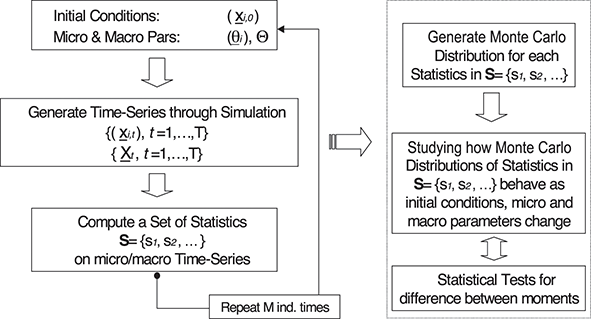
Figure 1 A schematic procedure for studying the output of an agent-based model.
Simulation exercises allow one then to study long-run statistical distributions, patterns, and emergent properties of micro and macro dynamics. For instance, a macro agent-based model can endogenously generate apparently ordered patterns of growth together with business cycles and deep crises. In that ABMs provide a direct answer to Solow and Stiglitz’s plea for macroeconomic models that can jointly account for long-run trajectories, short-run fluctuations, and deep downturns (see Section 1). At the same time, such models deliver a wealth of emergent properties ranging from macroeconomic relationships such as the Okun and Phillips curves to microeconomic distributions of, for example, firm size and growth rates, and so on. Moreover, as with every complex system, after crossing some critical threshold or tipping point the economy can self-organise along a different statistical path. This allows one to straightforwardly study phenomena like hysteresis in unemployment and GDP, systemic risk in credit, and financial markets, climate-change tipping points, and others.
More generally, the very structure of ABMs naturally allows one to take the model to the data and validate it against observed real-world observations. Most ABMs follow what has been called an indirect calibration approach (Windrum & Moneta, 2007; Fagiolo et al. 2017) which indeed represents also a powerful form of validation: the models are required to match a possibly wide set of micro and macro empirical regularities. An impressive list of micro and macro stylized facts jointly accounted by macro agent-based models is presented in Section 6; more in Haldane and Turrell (Reference Haldane and Turrell2019), Dosi et al. (Reference Dosi, Napoletano, Roventini and Treibich2016a) and Dosi et al. (Reference Dosi, Pereira, Roventini and Virgillito2020) among others. For instance, at the macro level, ABMs are able to match the relative volatility and comovements between GDP and different macroeconomic variables, the interactions between real, credit, and financial aggregates (including the emergence of deep banking crises), fat-tailed GDP growth-rate distributions, and so on. At the microeconomic level, macro agent-based models are able to reproduce firm size and growth rate distributions, heterogeneity and persistent differentials among firm productivity, lumpy investment patterns, and so on.
We do consider the ability of ABMs to jointly account for a huge ensemble of both micro and macro stylised facts under a wide range of parameterisations as the primary validation of their strength and robustness. In fact, it is relatively easy to ‘prove’ any model, no matter how far-fetched, concerning any one empirical regularity, in violation of all the rest we know about that particular phenomenon. So, for example, in the Middle Ages, there were astronomical theories apparently quite apt to ‘explain’ the day and the night in terms of God opening and closing the curtains of the universe. The analogy with DSGE models is striking indeed! However, the ABM perspective has accepted also such an epistemologically twisted comparative challenge and has made much progress even in terms of validation against a single time-series. A detailed survey with the most recent developments is provided in Fagiolo, Guerini, Lamperti et al. (Reference Fagiolo, Guerini, Lamperti, Moneta, Roventini, Beisbart and Saam2017).
On the ‘input side’, that is, modelling assumptions about individual ‘behaviours’ and interactions have been refined on laboratory experiments (Hommes, Reference Hommes2013; Anufriev, Bao, & Tuinstra, Reference Anufriev, Bao and Tuinstra2016), business practices (Dawid et al. Reference Dawid, Harting, van der Hoog and Neugart2019) and, more generally, microeconomic empirical evidence (Dosi et al., Reference Dosi, Napoletano, Roventini and Treibich2016a).Footnote 31 ABMs can also be validated on the output side, by explaining the space of parameters and initial conditions in terms of the range of values which allow the model to replicate the stylised facts of interest. For instance, Barde (Reference Barde2016) and Lamperti (Reference Lamperti2018) attempt to validate the output of agent-based models according to the replication of time-series dynamics, while Guerini and Moneta (Reference Guerini and Moneta2017) explore how a macro ABM matches the apparent causal relations in the data. Some works estimate ABMs via indirect inference (see e.g. Alfarano, Lux, & Wagner, Reference Alfarano, Lux and Wagner2005; Winker, Gilli, & Jeleskovic, Reference Winker, Gilli and Jeleskovic2007; Grazzini, Richiardi, & Sellad, Reference Grazzini, Richiardi and Sellad2013; Grazzini & Richiardi, Reference Grazzini and Richiardi2015) or Bayesian methods (Delli Gatti & Grazzini, Reference Delli Gatti and Grazzini2020; Grazzini, Richiardi, & Tsionas, Reference Grazzini, Richiardi and Tsionas2017). Finally, a new strand of research assesses the forecasting capabilities of ABMs vis-à-vis DSGE and VAR models (Poledna et al., Reference Poledna, Miess, Hommes and Rabitsch2023).
In any case, there is a fundamental distinction, often neglected by economists, between explanation and forecasting. One may well use clearly wrong theories in order to predict especially in the short term, and they might well be the ground for powerful heuristics for decision. Agent-based models of the K+S kind are primarily there with the ambition to explain. Together, they are also instrumental in showing the power of wrong models of prediction as robust guidance to behaviours in complex evolving environments. So in Dosi et al. (Reference Dosi, Napoletano, Roventini, Stiglitz and Treibich2020a), for example, one shows that the prediction rule ‘tomorrow will be likely today’ turns out to be a much more effective guidance for individual behaviours in complex and changing worlds than any more sophisticated inferential rule.
No matter the empirical validation procedures actually employed, an important domain of analysis regards the sensitivity of the model to parameter changes through different methods including Kriging meta-modeling (Salle & Yıldızoğlu,; Dosi, Pereira, & Virgillito, Reference Dosi, Pereira and Virgillito2017; Dosi et al., Reference Dosi, Pereira, Roventini and Virgillito2018a, Reference Dosi, Pereira, Roventini and Virgillito2018b; Bargigli et al., Reference Bargigli, Riccetti, Russo and Gallegati2020) and machine-learning surrogates (Lamperti, Roventini, & Sani, Reference Lamperti, Roventini and Sani2018). Such methodologies provide detailed sensitivity analyses of macro ABMs, allowing one to get a quite deep descriptive knowledge of the behaviour of the system, even concerning variables far from crucial for the general interpretative power of ABMs themselves. In this respect, however, note that, contrary to common wisdom, the most ‘important’ variables, whatever it means in a system rich of inter-relatedness, are those which are most insensitive to changes in parameterisations. What counts is primarily their presence or absence. This is the case, for example, of an innovation process of whatever kind, or a mechanism of demand generation, or a fiscal policy, again of whatever kind.
4.3 Policy Analysis
If empirically sound, agent-based models represent a very powerful device able to address policy questions under more realistic, flexible, and modular set-ups. Indeed, in contrast to DSGE models, they do not impose any strong theoretical consistency requirements (e.g., equilibrium, representative individual assumptions, rational expectations) and allow for behavioural assumptions which can be replaced in a modular way, without impairing the analysis of the model.Footnote 32 Moreover, as already mentioned earlier, agent-based models are able to jointly match a rich ensemble of macro and micro empirical regularities.This is a major advantage of ABMs vis-à-vis, for example, DSGE ones, which are typically built – in order to retain analytical solvability – to explain very few macro-stylised facts, and cannot replicate by construction any micro empirical regularities, given their representative-agent assumption.
But how can one actually conduct policy experiments in ABMs? In a very natural way, indeed. Take again the procedure for ABM descriptive analysis outlined in Figure 1. Micro and macro parameters can be designed in such a way to mimic real-world key policy variables like tax rates, subsidies, and others. Moreover, initial conditions might play a relevant role (somewhat equivalent to initial endowments in standard models) and describe different distributional set-ups concerning, for example, incomes or technologies. In addition, interaction and behavioural rules employed by economic agents can be easily devised so as to represent alternative institutional, market, or industry set-ups. Since all these elements can be freely interchanged, one can investigate a huge number of alternative policy experiments and rules, the consequences of which can be assessed either qualitatively or quantitatively (e.g., by running standard statistical tests on the distributions of the statistics in
 ). For example, one might statistically test whether the effect on the moments of the individual consumption distribution will be changed (and if so, by how much) by a percentage change in any given consumption tax rate. Most importantly, all this might be done while preserving the ability of the model to replicate existing macroeconomic stylized facts, as well as microeconomic empirical regularities, which by construction cannot be matched by DSGE models.
4.4 Conclusions
The number of macroeconomic agent-based models has steadily increased in the last decades, and this trend received a new impulse after the Great Recession uncovered many weaknesses of DSGE models. For instance, in their survey Dawid and Delli Gatti (Reference Dawid, Delli Gatti, Hommes and LeBaron2018) discuss eight families of macroeconomic agent-based models: the model of Ashraf, Gershman, and Howitt (Reference Ashraf, Gershman and Howitt2017), the Ancona–Milano approach (Delli Gatti et al., Reference Delli Gatti, Di Guilmi, Gaffeo, Giulioni, Gallegati and Palestrini2005; Assenza, Delli Gatti, & Grazzini, Reference Assenza, Delli Gatti and Grazzini2015), the Eurace@Unibi model (Dawid et al., Reference Dawid, Gemkow, Harting, van der Hoog, Neugart, Chen and Kaboudan2014a; Dawid, Harting, & Neugart, Reference Dawid, Harting and Neugart2014b, Reference Dawid, Harting and Neugart2018), the Eurace simulator developed in Genoa (Cincotti, Raberto, & Teglio, Reference Cincotti, Raberto and Teglio2010; Raberto et al., Reference Raberto, Ozel, Ponta, Teglio and Cincotti2019; Teglio et al., Reference Teglio, Mazzocchetti, Ponta, Raberto and Cincotti2019), the JAMEL model (Salle & Seppecher, Reference Salle and Seppecher2018; Seppecher, Reference Salle and Seppecher2018), the Keynes meeting Schumpeter model (Dosi, Fagiolo, & Roventini, Reference Dosi, Fagiolo and Roventini2010), the LAGOM model (Mandel, Jaeger, Fuerst et al., Reference Mandel, Jaeger, Fuerst, Lass, Lincke, Meissner, Pablo-Marti and Wolf2010; Wolf, Furst, Mandel et al., Reference Wolf, Furst, Mandel, Lass, Lincke, Pablo-Marti and Jaeger2013), and the model developed by Lengnick (Reference Lengnick2013). The list is not completely exhaustive. Among a burgeoning line of research, one should consider, for instance, the stock-flow consistent model by Caiani et al. (Reference Caiani, Godin, Caverzasi, Gallegati, Kinsella and Stiglitz2016), and the multi-industry models developed independently by Ciarli et al. (Reference Ciarli, Lorentz, Valente and Savona2019), Dosi, Roventini, and Russo (Reference Dosi, Roventini and Russo2019, Reference Dosi, Roventini and Russo2020), and Poledna et al. (Reference Poledna, Miess, Hommes and Rabitsch2023).
The surveys of Fagiolo and Roventini (Reference Fagiolo and Roventini2012, Reference Fagiolo and Roventini2017), Napoletano (Reference Napoletano2018), and Dawid and Delli Gatti (Reference Dawid, Delli Gatti, Hommes and LeBaron2018) show how macroeconomic agent-based models can succesfully address fiscal policy, monetary policy, macroprudential policy, labour-market governance, regional and cohesion policies, innovation and industrial policies, climate-change policies,Footnote 33 and different combinations of such public interventions. In that, ABMs are a valuable tool in the model portfolio available for policymakers as discussed by Haldane and Turrell (Reference Haldane and Turrell2019). An overview of such models is beyond the scope of the Element. On the contrary, in the next section, we will introduce the family of Keynes meeting Schumpeter models refining upon Dosi, Fagiolo, and Roventini (Reference Dosi, Fagiolo and Roventini2010), which can be considered our workhorse ABM accounting for macro and micro dynamics, as well as for testing the impact of different combinations of microeconomic and macroeconomic policies.
5 The Schumpeter Meeting Keynes Model
The Schumpeter meeting Keynes (K+S) family of agent-based models (Dosi, Fagiolo & Roventini Reference Dosi, Fagiolo and Roventini2010; Dosi et al. Reference Dosi, Fagiolo, Napoletano and Roventini2013, Reference Dosi, Fagiolo, Napoletano, Roventini and Treibich2015, Reference Dosi, Pereira, Roventini and Virgillito2017, Reference Dosi, Pereira, Roventini and Virgillito2018a, Reference Dosi, Pereira, Roventini and Virgillito2019, Reference Dosi, Napoletano, Roventini, Stiglitz and Treibich2020a) is able to jointly account for endogenous growth and business fluctuations punctuated by major crises.Footnote 34 In that, it responds to the pleas of Solow (Reference Solow2005) and Stiglitz (Reference Stiglitz2011) to design models that knit together short- and long-run dynamics, as well as are able to account for rare deep downturns. Beyond that, the K+S model reproduces a rich list of macro and micro stylised facts and it can be employed as a laboratory to test the short- and long-run impact of different ensembles of innovation, industrial, fiscal, and monetary policies.
Rooted in the evolutionary (Nelson & Winter, Reference Nelson and Winter1982, see also Dosi et al., Reference Dosi, Freeman, Nelson, Silverberg and Soete1988) and agent-based (cf. Tesfatsion, Reference Tesfatsion, Tesfatsion and Judd2006) perspectives, the K+S model addresses five major, interrelated, questions. First, it investigates the processes by which technological innovations affect macro variables such as unemployment rates and, in the longer term, output growth rates.
Together with this ‘Schumpeterian’ question, second, we ask how such endogenous changes in the ‘fundamentals’ of the economy interact with demand conditions. This is a basic ‘Keynesian’ question. How does aggregate demand modulate the diffusion and the macro impact of technological innovations? And, conversely, how does it affect, if at all, the amount of search and the degree of exploitation of innovation opportunities themselves?
Third, we explore long-term effects of demand conditions. Is the long-term growth just driven by changes in the technological ‘fundamentals’? Or, can variations in aggregate demand influence future dynamics?
Four, the K+S model investigates the interactions between the real and financial sides of the economy, thus reproducing the Minskian features of business cycles (Minsky, Reference Minsky1986) and the endogenous emergence of banking crises.
Fifth, it allows the exploitation of the properties and impact of different arrangements in the institutions governing labour relations, including the way labour markets operate, and wages are set.
Sixth, it allows the study of the intrinsic duality of technological change with its labour-shedding effect via productivity improvements, on the one side, and the job-creating effect via the introduction of new products, on the other.
The fully fledged version of the K+S model describes an economy with heterogeneous firms – belonging either to a capital- or consumption-good industry – banks, a labour force, a central bank, and a government (see Figure 2). Innovation and imitation routines performed by capital-goods firms investing in R&D drive the process of technical change, resulting in cheaper and far more productive machines sold to the consumption-goods sector. The latter firms produce (in the baseline version of the model) a homogeneous final good and may use external financing from the banking sector if their internal resources do not cover production and investment expenses. Both firms and banks can go bankrupt if their net worth becomes negative, possibly triggering a crisis. The government fixes taxes and unemployment subsidy rates and bails out bankrupted banks. The central bank sets the baseline interest rate for the economy.
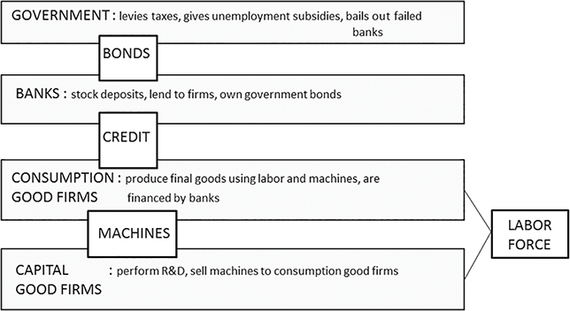
Figure 2 A schematic representation of the Schumpeter meeting Keynes (K+S) model.
In what follows, we present the basic K+S model and its credit-market and labour-market extensions. The empirical validation of the model will be reported in Section 6. Finally, the policy experiments will be presented in Section 7.
5.1 The Timeline of Events
As already mentioned, our simple economy is composed of a machine-producing sector made of
 firms (denoted by the subscript
 ), a consumption-good sector made of
 firms (denoted by the subscript
 ),
),
 consumers/workers, and a public sector. Before accurately describing the K+S model (Dosi, Fagiolo, & Roventini, Reference Dosi, Fagiolo and Roventini2010), we briefly provide the timeline of events occurring in each time step (
 ).
).
1. Machine-tool firms perform R&D trying to discover new products and more efficient production techniques and to imitate the technology and the products of their competitors.
2. Capital-good firms advertise their machines with consumption-good producers.
3. Consumption-good firms decide how much to produce and invest. If investment is positive, consumption-good firms choose their supplier and send their orders, for their planned expansion, and, possibly, also to replace some older equipments.
4. In both industries firms hire workers according to their production plans and start producing.
5. Imperfectly competitive consumption-good market opens. The market shares of firms evolve according to their ‘competitiveness’ based on prices and possibly other variables such as any unfilled demand.
6. Entry and exit take places. In both sectors firms with near-zero market shares and negative net liquid assets are eschewed from the two industries and replaced by new firms.
7. Machines ordered at the beginning of the period are delivered and become part of the capital stock at time
 .
.

At the end of each time step, aggregate variables (e.g. GDP, investment, employment) are computed, summing over the corresponding microeconomic variables.
Let us now turn to a more detailed description of the model and of the agents’ behaviours, which – to repeat –we try to keep as close as we can to what we know they actually do as distinct from what they ought to do under more perfect informational circumstances.
5.2 The Capital-Good Industry
The technology of a capital-good firm is
 , where the former coefficient stands for the labour productivity of the machine-tool manufactured by
 for the consumption-good industry (a rough measure of producer quality), while the latter coefficient is the labour productivity of the production technique employed by firm
 itself. The positive integer
 denotes the current technology vintage. Given the monetary wage
 , the unit cost of production of capital-good firms is:
 (1)
(1)
With a fixed mark-up (
 ) pricing rule,Footnote 35 prices (
 ) are defined as:
 (2)
(2)
The unit labour cost of production in the consumption-good sector associated with each machine of vintage
 , produced by firm
 is:
is:

Firms in the capital-good industry ‘adaptively’ strive to increase their market shares and their profits trying to improve their technology both via innovation and imitation. Both are costly processes: firms invest in R&D a fraction of their past sales (
 ):
):
 (3)
(3)
with
 . R&D expenditures are employed to hire researchers paying the market wage
 .Footnote 36 Firms split their R&D efforts between innovation (
 ) and imitation (
 ) according to the parameter
 :
:

We model innovation as a two-step process. The first one determines whether a firm obtains or not an access to innovation – irrespectively of whether it is ultimately a success or a failure – through a draw from a Bernoulli distribution, whose parameter
 is given by:
 (4)
(4)
with  capturing firms’ search capabilities. Note that according to (4), there are some scale-related returns to R&D investment: access to innovative discoveries is more likely if a firm puts more resources into R&D. If a firm innovates, it may draw a new machine embodying technology
 according to:

where
 and
and
 are two independent draws from a Beta(
 ) distribution over the support
 with
with
 belonging to the interval
 and
and
 to
to
 . Note that the notional possibilities of technological advance – namely technological opportunities (Dosi, Reference Dosi2023) – are captured by the support of the Beta distribution and by its shape. So, for example, with low opportunities the largest probability density falls over ‘failed’ innovations – that is, potential capital goods which are ‘worse’ in terms of costs and performances than those already produced by the searching firm. Conversely, under a condition of rich opportunities, innovations which dominate incumbent technologies will be drawn with high probability. As we shall show later in the Element, a crucial role of ‘Schumpeterian’ technology policies is precisely to influence opportunities and micro capabilities.
Like innovation search, imitation follows a two-step procedure. The possibilities of accessing imitation come from sampling a Bernoulli, (
 ):
):
 (5)
(5)
with
 . Firms accessing the second stage are able to copy the technology of one of the competitors
 . We assume that firms are more likely to imitate competitors with similar technologies and we use a Euclidean metric to compute the technological distance between every pair of firms to weight imitation probabilities. Such appropriability conditions stem from the tacit nature of knowledge embodied in the technology, even in the presence of explicit intellectual properties rights (which, however, can be easily modeled in our framework).
All firms which draw a potential innovation or imitation have to put it on production or keep producing the incumbent generation of machines. Comparing the technology competing for adoption, firms choose to manufacture the machine characterised by the best trade-off between price and efficiency. More specifically, knowing that consumption-good firms invest following a payback period routine (see Section 5.3), capital-good firms select the machine to produce according to the following rule:

where
 is a positive payback period parameter (see Eq. 10). Once the type of machine is chosen, we capture the imperfect information pervading the market, assuming that each firm sends a ‘brochure’ with the price and the productivity of its offered machines to both its historical (
 ) clients and to a random sample of potential new customers (
 ), whose size is proportional to
 (i.e.,
 , with
 ).
).
5.3 The Consumption-Good Industry
Consumption-good firms produce a homogenous goods using capital (i.e. their stock of machines) and labour under constant returns to scale. Firms plan their production (
 ) according to adaptive demand expectations (
 ):
):
 (7)
(7)
where
 is the demand actually faced by firm
 at time
 (
(
 positive integer).Footnote 37 The desired level of production (
 ) depends on the expected demand as well as on the desired inventories (
 ) and the actual stock of inventories (
 ):
):
 (8)
(8)
with
 . The output of consumption-good firms is constrained by their capital stock (
 ). If the desired capital stock (
 ) – computed as a function of the desired level of production – is higher than the current capital stock, firms invest (
 ) in order to expand their production capacity:Footnote 38
 (9)
(9)
The capital stock of each firm is obviously composed of heterogenous vintages of machines with different productivity. We define
 as the set of all vintages of machine-tools belonging to firm
 at time
 . Firms scrap machines following a payback period routine. Consequently, technical change and equipment prices influence the replacement decisions of consumption-good firms.Footnote 39 More specifically, firm
 replaces machine
 according to its technology obsolescence as well as the price of new machines:
 (10)
(10)
where
 and
and
 are the price and unit cost of production upon the new machines. Firms compute their replacement investment by summing up the number of old machine-tools, satisfying Eq. 10. Moreover, they also scrap the machines older than
 periods (with
 being a positive integer).
Consumption-good firms choose their capital-good supplier by comparing the price and productivity of the currently manufactured machine-tools they are aware of. As we mentioned earlier (see Section 5.2), the capital-good market is systematically characterised by imperfect information. This implies that consumption-good firms compare ‘brochures’ describing the characteristics of machines only from a subset of equipment suppliers. Firms then choose the machines with the lowest price and unit cost of production (i.e.,
 and send their orders to the corresponding machine manufacturer. Machine production is a time-consuming process: capital-good firms deliver the ordered machine-tools at the end of the period.Footnote 40 Gross investment of each firm (
 ) is the sum of expansion and replacement investment. Pooling the investment of all consumption-good firms, one gets aggregate investment (
 ).
).
Consumption-good firms have to finance their investments, as well as their production, as they advance worker wages. In line with any empirical observation and also a growing number of theoretical and empirical papers (e.g. Stiglitz & Weiss, Reference Stiglitz and Weiss1992; Greenwald & Stiglitz, Reference Greenwald and Stiglitz1993a; Hubbard, Reference Hubbard1998), we assume imperfect capital markets. This implies that the financial structure of firms matters (external funds are more expensive than internal ones) and firms may be credit rationed. More specifically, consumption-good firms finance production using their stock of liquid assets (
 ). If liquid assets do not fully cover production costs, firms borrow the remaining part, paying an interest rate
 up to a maximum debt/sales ratio of
 . Only firms that are not production-rationed can try to fulfill their investment plans by employing their residual stock of liquid assets first and then their residual borrowing capacity.Footnote 41
Given their current stock of machines, consumption-good firms compute average productivity (
 ) and unit cost of production (
 ). Prices are set applying a variable mark-up (
 ) on unit costs of production:
 (11)
(11)
Mark-up variations are regulated by the evolution of firm market shares (
 ):Footnote 42
 (12)
(12)
with
 .
.
The consumption-good market too is characterized by imperfect information (antecedents in the same vein are Phelps and Winter, Reference Phelps, Winter and Phelps1970; Klemperer, Reference Klemperer1987; Farrel & Shapiro, Reference Farrel and Shapiro1988; see also the empirical literature on consumers’ imperfect price knowledge surveyed in Rotemberg, Reference Rotemberg2008). This implies that consumers do not instantaneously switch to products made by more competitive firms. However, prices are clearly one of the key determinants of firms’ competitiveness (
 ). The other component is the level of unfilled demand (
 ) inherited from the previous period:
 (13)
(13)
where
 are positive parameters.Footnote 43 Weighting the competitiveness of each consumption-good firm by its past market share (
 ), one can compute the average competitiveness of the consumption-good sector:

This variable represents also a moving selection criterion driving, other things being equal, expansion, contraction, and extinction within the population of firms. We parsimoniously model this market set-up, letting firm market shares evolve according to a ‘quasi’ replicator dynamics (for antecedents in the evolutionary camp see Metcalfe, Reference Metcalfe1994a; Silverberg, Dosi, & Orsenigo, Reference Silverberg, Dosi and Orsenigo1988):
 (14)
(14)
with
 Footnote 44
The profits (
 ) of each consumption-good firm reads:

where
 and
and
 denotes the stock of debt. The investment choices of each firm and its profits determine the evolution of its stock of liquid assets (
 ):
):

where
 is the amount of internal funds employed by firm
 to finance investment.
5.4 Schumpeterian Exit and Entry Dynamics
At the end of each period, we let firms with (quasi) zero market shares or negative net assets die and we allow a new breed of firms to enter the markets. In many of our models, we keep the number of firms fixed, hence any dead firm is replaced by a new one (this simplifying assumption is, however, by no means a necessary one).
In line with the empirical literature on firm entry (Caves, Reference Caves1998; Bartelsman, Scarpetta, & Schivardi, Reference Bartelsman, Scarpetta and Schivardi2005), we assume that entrants are on average smaller than incumbents, with the stock of capital of new consumption-good firms and the stock of liquid assets of entrants in both sectors being a fraction of the average stocks of the incumbents. More specifically, the stock of capital of a new consumption-good firm is obtained by multiplying the average stock of capital of the incumbents by a random draw from a Uniform distribution with support
 . In the same manner, the stock of liquid assets of an entrant is computed by multiplying the average stock of liquid assets of the incumbents of the sector by a random variable distributed according to a Uniform distribution with support
 .
.
Concerning the technology of entrants, new consumption-good firms select amongst the newest vintages of machines according to the ‘brochure mechanism’ described earlier. The process- and product-related knowledge of new capital-good firms is again drawn from a Beta distribution, whose shape and support are shifted and ‘twisted’ according to whether entrants enjoy an advantage or a disadvantage vis-à-vis incumbents. More precisely, the technology of capital-good firms is obtained by applying a coefficient extracted from a Beta(
 ) distribution to the endogenously evolving technology frontier (
 , where
 and
and
 are the best technology available to incumbents. In fact, the distribution of opportunities for entrants versus incumbents is a crucial characteristic of different sectoral technological regimes (a particular case of that is the distance from the technological frontier of entrants discussed in Aghion & Howitt, Reference Aghion and Howitt2007).
5.5 The Labour Market
The labour market is certainly not Walrasian: real wages not claring the market and involuntary unemployment as well as labour rationing are the rules rather than the exceptions. The aggregate labour demand (
 ) is computed by summing up the labour demand of capital- and consumption-good firms. The aggregate supply (
 ) is exogenous and inelastic. Hence aggregate employment (
 ) is the minimum between
 and
and
 .
.
The wage rate is determined by institutional and market factors. In the simplest case, which we use in our baseline version, wages are determined at the macro level via indexation mechanisms upon consumption prices and average productivity, on the one hand, and adjustments to unemployment rates, on the other:
 (15)
(15)
where
 is the average labour productivity,
 is the consumer price index, and
 is the unemployment rate. Variations may be experimented with, mimicking different regimes for the labour market, by changing the system parameters
 . However, more adequate representations of different regimes in a genuine ABM spirit are required. We present some promising attempts in Section 5.8. In any case, note that the analogy between Eq. 15 and any form of ‘Phillips curve’ is only superficial. Indeed, our results hold even if the coefficient on the unemployment term is set to zero. The importance of the relation is in terms of the transmission process from productivity to wages (or the absence thereof).
5.6 Consumption, Taxes, and Public Expenditures
An otherwise black-boxed public sector levies taxes on firm profits and worker wages or on profits only and pays to unemployed workers a subsidy (
 ) that is a fraction of the current market wage (i.e.,
 , with
 ). In fact, taxes and subsidies are the fiscal leverages that contribute to the aggregate demand management regimes (we shall explore this issue in more detail later). Note that a ‘zero tax, zero subsidy’ scenario is our benchmark for a pure Schumpeterian regime of institutional governance (see the experiments in Section 7).
Aggregate consumption (
 ) is computed by summing up over the income of both employed and unemployed workers:
 (16)
(16)
The model satisfies the standard national account identities: the sum of value added of capital- and consumption goods firms (
 ) equals their aggregate production since in our simplified economy there are no intermediate goods, and that in turn coincides with the sum of aggregate consumption, investment, and change in inventories (
 ):
):

The dynamics generated at the micro level by decisions of a multiplicity of heterogenous, adaptive agents and by their interaction mechanisms is the explicit microfoundation of the dynamics for all aggregate variables of interest (e.g. output, investment, employment). However, as the model amply demonstrates, the aggregate properties of the economy do not bear any apparent isomorphism with the micro adjustment rules outlined earlier. Needless to say, a fundamental consequence is also that any ‘representative agent’ compression of micro heterogeneity is likely to offer a distorted account of both what agents do and the collective outcomes of their actions – more in Dosi (Reference Dosi2023), indeed, well in tune with the arguments of Kirman (Reference Kirman1992) and Solow (Reference Solow2008).
5.7 The Credit Market Extensions
Building on the initial set-up presented and tested in Dosi, Fagiolo & Roventini (Reference Dosi, Fagiolo and Roventini2010), the model has been extended (Dosi et al., Reference Dosi, Fagiolo, Napoletano and Roventini2013, Reference Dosi, Fagiolo, Napoletano, Roventini and Treibich2015), introducing a credit market populated by heterogenous banks in order to study the possible interplays between the real and financial sectors. Such addition allows us to investigate the role of credit in amplifying and triggering macroeconomic fluctuations, possibly leading to the emergence of bank and sovereign debt crises and deep downturns that could affect the long-run performance of the economy (see Levine, Reference Levine1997: explicitly opposing Schumpeter’s view on that). The credit sector is populated by
 heterogenous banks, which gather deposits, distribute loans, and own sovereign bonds. In addition, a central bank now sets the baseline interest rate following a Taylor rule.
Banks are heterogenous in their number of clients (drawn from a Pareto distribution). Credit supply is constrained by capital adequacy requirements inspired by Basel-framework rules. Besides the regulatory limit, we assume that banks maintain a buffer over the regulatory capital level, as indicated by the empirical evidence (BIS, 1999). The size of such buffers evolves strategically in order to offset bank financial fragility along the business cycle, and it is proxied by the ratio between accumulated bad debt (i.e. loans in default) and bank assets (i.e. sum of the stocks of loans, sovereign bonds, and reserves held by the bank),
 . Total credit supply available from bank
 at time
 therefore is as follows:
 (17)
(17)
where
 is a parameter that measures the banks’ speed of adjustment to its financial fragility, and
 is the macroprudential regulatory parameter. Credit supply therefore decreases in
 and
and
 and is positively affected by banks’ equity.
Banks allocate credit across firms by ranking them according to their creditworthiness, proxied by the ratio between firms’ past net worth and sales. Loans are granted to firms as long as credit supply is not exhausted. As a consequence, consumption-goods firms may be credit-rationed. Firms’ probability to get a loan depends on their credit ranking as well as on the financial health of their bank. Note that the lower performance of other clients improves firms’ relative ranking, but also has a negative impact on total credit availability, because firms’ defaults weaken the equity of their bank, thus reducing the supply of credit.
We assume that the central bank follows a Taylor rule, which adjusts the interest rate to changes in inflation and, under some revealing policy scenarios, to unemployment, relative to their target levels:
 (18)
(18)
where
 is the inflation rate of the period,
 the unemployment rate, and
 are the target interest, inflation, and unemployment rates, respectively. Banks fix the interest rate on loans by applying a risk premium on the policy rate.
Bank revenues are composed of interests from loans, deposits at the central bank, and sovereign bonds. Gross profits are taxed at the rate
 . Massive loan losses may turn profits negative, reducing the equity of banks and their credit supply. A bank goes bankrupt if firm bankruptcy shocks turn its net worth negative. In such a case, the government steps in and recapitalizes the bank. The public bailout entails a cost (
 ), equal to the difference between the equity of the failed bank before and after the intervention, which affects the public budget.
Given government tax revenues (
 ) and expenses, public deficit reads:
 (19)
(19)
where
 are unemployment subsidies and
 is the cost of sovereign debt. Deficits are financed on the bonds market, where banks buy the bonds issued by the government. Banks buy bonds with their net profits; if the total bank savings are lower than the stock of sovereign debt that needs to be refinanced, the central bank buys the residual part.
5.8 The Labour-Market Extension
A series of our contributions (Dosi et al., Reference Dosi, Pereira, Roventini and Virgillito2017, Reference Dosi, Pereira, Roventini and Virgillito2018a, Reference Dosi, Pereira, Roventini and Virgillito2018b, Reference Dosi, Pereira, Roventini and Virgillito2019, Reference Dosi, Freeman, Pereira, Roventini and Virgillito2021) have extended the K+S model, accounting for decentralised interactions in the labour market between heterogenous workers and firms. Such interactions occur within different institutions characterising wage-setting rules and labour markets, for example the presence (or not) of minimum wage, unemployment subsidy, firing rules, and so on.
The aggregate supply of labour
 is still fixed, while the desired labour demand
 by any consumption-good firm
 is determined by the ratio between the desired production
 and the average productivity of its current capital stock
 (see Section 5.3):
 (20)
(20)
A similar process is performed by firms
 in the capital-good sector to define
 , considering effective orders
 and labour productivity in the current machine-producing technique
 .Footnote 45 Given the existing labour force of the firm
 , the desired variation of employment
 is then calculated as follows:
 (21)
(21)
Each firm
 gets, in probability, a fraction of the applicant workers in its ‘candidates queue’, proportional to its market share
 :
:
 (22)
(22)
where
 is a parameter defining the number of job ‘queues’ each seeker joins, in average, and
 is the expected number of workers in the queue of firm
 . As workers can apply to more than one firm at a time, firms may not be able to hire all workers in their queue, even when they mean to. Considering the set of workers in the candidates queue
 , each firm has to select to whom to make a job (wage) offer. The set of desired workers
 , among those in the queue
 , is defined as:
 (23)
(23)
that is, the firm targets workers that would accept its wage offer
 , considering the wage
 requested (if any), up to its demand of workers
 . Therefore, the number of effectively hired workers (the size of set
 ) is:
) is:
 (24)
(24)
The model allows for different institutional regimes in the labour market. In the first one, which we call ‘Fordist’, there is an implicit pact among firms and workers, implying that the latter never voluntarily quit their jobs, while firms fire employees (
 ) only when experiencing negative profits
 and shrinking production
 . Of course, firms exiting the market always fire all their workers. Conversely, only unemployed workers search for jobs.Footnote 46
Wages are not bargained. Firm
 unilaterally offers a wage
 based on past offers according to the following rule:
 (25)
(25)
The wage premium
 is defined as:
 (26)
(26)
with
 being the aggregate labour productivity,
 the firm-specific productivity, and
 the parameters. The gains in labour productivity are then passed to workers via wage increases. Moreover, wages are linked not only to firm-specific performance but also to the aggregate productivity dynamics of the economy. Finally, note that
 is simultaneously applied to all existing workers of firm
 , so there is no intra-firm differential in wages.Footnote 47
Another archetype we study is the ‘Competitive’ regime, which can result from the introduction of structural reforms to spur flexibility in the labour market. In the new setting, wages adjust to labour market conditions: firms freely hire and fire in each period, and employees can actively search for better jobs all the time.
The wage
 requested by worker
 is a function of the individual unemployment condition and the past wage history. If the worker was unemployed in the previous period, the requested
 shrinks. More specifically, she will ask for the maximum between the unemployment benefit
 (if available) and her own satisfying wage
 :
:
 (27)
(27)
with the parameter
 . The satisfying wage accounts for the recent wage history:

that is, as the moving average salary of the last
 periods.
Considering job applications and knowing the required number of workers
 to hire, the wage offered by each firm is the minimum that satisfies enough workers in its queue
 . So, it is the highest wage requested by the cheapest available workers which fulfils
 :
:
 (30)
(30)
Employed workers search for better-paid jobs in each period. If a worker gets an offer from another firm
 , she decides whether to quit or not from her current employer
 if
if
 . That is, worker
 quits firm
 if she receives a wage offer
 from at least one firm
 that is equal or higher than her required wage
 .
.
Note that, differently from the original version of the K+S model, the market wage is not determined by exogenous institutional factors (see Equation 15), but it is microfounded via the local interactions of heterogeneous firms and workers. The unemployed benefit
 is a fraction of the current average wage:
 (31)
(31)
where
 is a parameter and
 , the past period average wage. The government can also fix an institutional minimum wage
 which imposes a lower bound to the firm-specific wage-setting behaviour:
 (32)
(32)
6 Empirical Validation
The Keynes+Schumpeter model does not allow for analytical, closed-form solutions. As discussed in detail in Section 4, this general ABM distinctive feature stems from the non-linearities present in agent decision rules and their interaction patterns, and it forces us to run computer simulations to analyse the properties of the stochastic processes governing the coevolution of micro and macro variables. In order to do so, the K+S model can be developed in the Laboratory for Simulation Development (LSD) platform (Valente, Reference Valente2008), a free, open-source, user-friendly software framework dedicated to agent-based models. The online Appendix written by Marcelo C. Pereira (University of Campinas) provides all the steps to produce and analyse the results from the original Schumpeter meeting Keynes (K+S) model.Footnote 48 One can then perform extensive Monte Carlo simulation analyses to wash away across-simulation variability. As a consequence, the results presented in this section and the next one typically refer to across-run averages over one hundred replications and their standard-error bands.Footnote 49
To begin with, we study whether the family of K+S models are able to reproduce jointly a wide range of macroeconomic and microeconomic stylised facts (SF, the ‘benchmark’ parametrisation is reported in Tables A.1 and A.2 Appendix A).Footnote 50 As mentioned earlier, if the K+S models successfully match empirical regularities concerning industrial dynamics as well as more structural relations between macroeconomic aggregates, this ought to be taken as a robust empirical validation (Fagiolo et al., Reference Fagiolo and Roventini2017; Fagiolo & Roventini, Reference Fagiolo, Guerini, Lamperti, Moneta, Roventini, Beisbart and Saam2017), lending plausibility to its use as a ‘computational laboratory’ to test different policy experiments. We report in Tables 1 and 2 the list of macro and micro empirical regularities that the K+S model is able to account for (which include those discussed by Haldane & Turrell, Reference Haldane and Turrell2019). Note, to repeat, that the fact that a large number of very different micro and macro stylized facts are reproduced by the model makes our empirical validation exercises far more demanding than a simple polynomial-fitting exercise in the presence of some free parameters. At the same time, our macro agent-based model is able to account for a rich list of micro empirical regularities which cannot be structurally matched by any DSGE model given their representative-agent ‘microfoundations’.
Table 1 Macroeconomic stylised facts replicated by the K+S model.
| Stylised facts | Empirical studies (among others) | |
|---|---|---|
| SF1 | Endogenous self-sustained growth with persistent fluctuations | Burns and Mitchell (Reference Burns and Mitchell1946); Kuznets and Murphy (Reference Kuznets and Murphy1966); Stock and Watson (Reference Stock, Watson, Taylor and Woodford1999); Zarnowitz (Reference Zarnowitz1985) |
| SF2 | Fat-tailed GDP growth-rate distribution | Castaldi and Dosi (Reference Castaldi and Dosi2009); Fagiolo, Napoletano, and Roventini (Reference Fagiolo, Napoletano and Roventini2008) |
| SF3 | Recession duration exponentially distributed | Ausloos, Miskiewicz, and Sanglier (Reference Ausloos, Miskiewicz and Sanglier2004); Wright (Reference Wright2005) |
| SF4 | Relative volatility of GDP, consumption and investment | Stock and Watson (Reference Stock, Watson, Taylor and Woodford1999) Napoletano, Roventini, and Sapio (Reference Napoletano, Roventini and Sapio2006) |
| SF5 | Cross-correlations of macro variables | Napoletano, Roventini, and Sapio (Reference Napoletano, Roventini and Sapio2006); Stock and Watson (Reference Stock, Watson, Taylor and Woodford1999) |
| SF6 | Pro-cyclical aggregate R&D investment | Walde and Woitek (Reference Walde and Woitek2004) |
| SF7 | Cross-correlations of credit-related variables | Leary (Reference Leary2009); Lown and Morgan (Reference Lown and Morgan2006) |
| SF8 | Cross-correlation between firm debt and loan losses | Foos, Norden, and Weber (Reference Foos, Norden and Weber2010); Mendoza and Terrones (Reference Mendoza and Terrones2012) |
| SF9 | Banking crises duration is right skewed | Reinhart and Rogoff (Reference Reinhart and Rogoff2009) |
| SF10 | Fiscal costs of banking crises to GDP distribution is fat-tailed | Laeven and Valencia (Reference Laeven and Valencia2008) |
| SF11 | Beveridge curve | |
| SF12 | Okun curve | |
| SF13 | Wage curve | |
| SF14 | Matching function | |
| SF15 | Endogenous volatility of productivity, unemployment, vacancy, separation, and hiring rates | Shimer (Reference Shimer2005) |
Table 2 Microeconomic stylised facts replicated by the K+S model.
| Stylised facts | Empirical studies (among others) | |
|---|---|---|
| SF16 | Firm (log) size distribution is right-skewed | Dosi (Reference Dosi, Malerba and Brusoni2007) |
| SF17 | Fat-tailed firm growth-rate distribution | Bottazzi and Secchi (Reference Bottazzi and Secchi2003, Reference Bottazzi and Secchi2006) |
| SF18 | Productivity heterogeneity across firms | Bartelsman and Doms (Reference Bartelsman and Doms2000); Dosi (Reference Dosi, Malerba and Brusoni2007) |
| SF19 | Persistent productivity differential across firms | Bartelsman and Doms (Reference Bartelsman and Doms2000); Dosi (Reference Dosi, Malerba and Brusoni2007) |
| SF20 | Lumpy investment rates at firm-level | Doms and Dunne (Reference Doms and Dunne1998) |
| SF21 | Firm bankruptcies are counter-cyclical | Jaimovich and Floetotto (Reference Jaimovich and Floetotto2008) |
| SF22 | Firm bad-debt distribution fits a power-law | Di Guilmi, Gallegati, and Ormerod (Reference Di Guilmi, Gallegati and Ormerod2004) |
| SF23 | Fat-tailed unemployment time distribution | |
| SF24 | Fat-tailed wage growth-rate distribution | |
| SF25 | Heterogenous skill distribution | |
6.1 Macroeconomic Empirical Regularities
The macroeconomic empirical regularities matched by the K+S model are reported in Table 1. First, the generated time series show the emergence of endogenous self-sustained economic growth with persistent fluctuations (SF1, see Figure 3). Business cycles are punctuated by deep downturns (Stiglitz, Reference Stiglitz2014) and, in line with the empirical evidence (e.g. Fagiolo, Napoletano & Roventini Reference Fagiolo, Napoletano and Roventini2008; Ascari, Fagiolo, & Roventini, Reference Ascari, Fagiolo and Roventini2015), the GDP growth-rate distribution exhibits fat tails (SF2, see Figure 4), revealing the coexistence of mild and deep downturns. Moreover, most recessions are short-lived; few last for long periods of time. The distribution of the duration of recessions generated by the model is exponential (SF3, see Figure 5), as found in empirical data (Ausloos, Miskiewicz, & Sanglier, Reference Ausloos, Miskiewicz and Sanglier2004; Wright, Reference Wright2005).
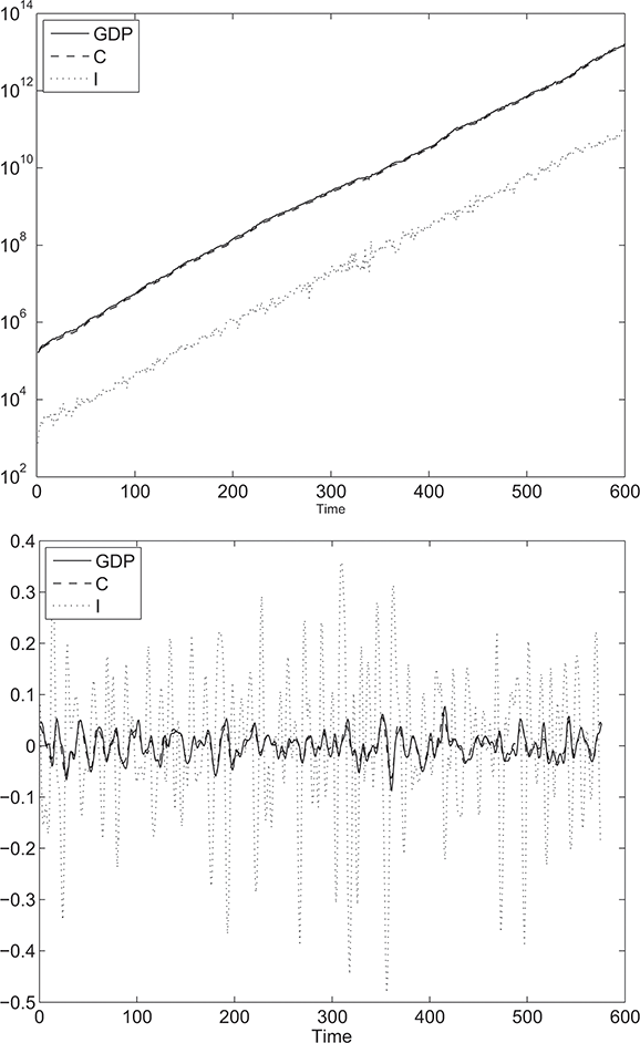
Figure 3 Output, consumption, and investment time series; top: logs; bottom: bandpass-filtered (6,32,12) series, reproduced from Dosi et al. (Reference Dosi, Fagiolo, Napoletano, Roventini and Treibich2015).
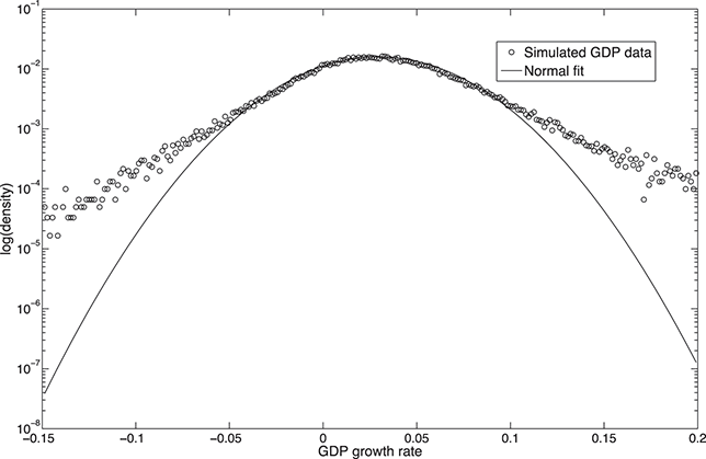
Figure 4 Distribution of real GDP growth rates: binned simulated densities (250 bins, 59,900 observations, circles) vs. normal fit (Dosi et al., Reference Dosi, Fagiolo, Napoletano, Roventini and Treibich2015).
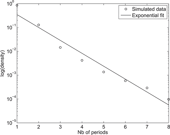
Figure 5 Exponential fit of recession durations (Dosi et al., Reference Dosi, Fagiolo, Napoletano, Roventini and Treibich2015).
We then de-trend the macroeconomics series to study their behaviour at the business cycle frequencies. Well in tune with the empirical evidence (e.g. Stock & Watson, Reference Stock, Watson, Taylor and Woodford1999; Napoletano, Roventini & Sapio, Reference Napoletano, Roventini and Sapio2006), the fluctuations of aggregate consumption are smoother than those of GDP, whereas investment is more volatile than output (SF4, see Figure 3, bottom). Moreover, the co-movements between GDP and the most important macroeconomic variables are in line with what is found in real data (SF5, see Table 3): consumption is pro-cyclical and coincident; net investment, changes in inventories, productivity, nominal wages, and inflation are pro-cyclical; unemployment, prices, and mark-ups are counter-cyclical; the real wage is acyclical.Footnote 51 Finally, R&D investment is pro-cyclical (SF6; see e.g. Walde & Woitek, Reference Walde and Woitek2004).
Table 3 Correlation structure. Bpf: bandpass-filtered (6,32,12) series. Monte Carlo simulation standard errors in parentheses.
| Series | Output (Bpf) | ||||||||
|---|---|---|---|---|---|---|---|---|---|
| (Bpf) | t−4 | t−3 | t−2 | t−1 | t | t+1 | t+2 | t+3 | t+4 |
| Output | −0.1022 | 0.1769 | 0.5478 | 0.8704 | 1 | 0.8704 | 0.5478 | 0.1769 | −0.1022 |
| (0.0090) | (0.0080) | (0.0048) | (0.0014) | (0) | (0.0014) | (0.0048) | (0.0080) | (0.0090) | |
| Consumption | −0.1206 | 0.0980 | 0.4256 | 0.7563 | 0.9527 | 0.9248 | 0.6848 | 0.3394 | 0.0250 |
| (0.0123) | (0.0129) | (0.0106) | (0.0062) | (0.0017) | (0.0018) | (0.0038) | (0.0058) | (0.0072) | |
| Investment | −0.2638 | −0.3123 | −0.2646 | −0.0864 | 0.1844 | 0.4473 | 0.5950 | 0.5757 | 0.4206 |
| (0.0102) | (0.0137) | (0.0182) | (0.0210) | (0.0206) | (0.0175) | (0.0139) | (0.0123) | (0.0129) | |
| Net Investment | −0.0838 | 0.0392 | 0.2195 | 0.4010 | 0.5114 | 0.5037 | 0.3850 | 0.2105 | 0.0494 |
| (0.0122) | (0.0167) | (0.0216) | (0.0235) | (0.0211) | (0.0153) | (0.0103) | (0.0112) | (0.0138) | |
| Ch. in Invent. | 0.0072 | 0.1184 | 0.2349 | 0.2948 | 0.2573 | 0.1331 | −0.0199 | −0.1319 | −0.1640 |
| (0.0081) | (0.0070) | (0.0060) | (0.0072) | (0.0090) | (0.0098) | (0.0097) | (0.0085) | (0.0067) | |
| Employment | −0.3240 | −0.1901 | 0.0796 | 0.4083 | 0.6692 | 0.7559 | 0.6451 | 0.4067 | 0.1555 |
| (0.0087) | (0.0123) | (0.0151) | (0.0160) | (0.0149) | (0.0120) | (0.0084) | (0.0069) | (0.0082) | |
| Unempl. Rate | 0.3357 | 0.2084 | −0.0596 | −0.3923 | −0.6607 | −0.7550 | −0.6489 | −0.4112 | −0.1583 |
| (0.0083) | (0.0118) | (0.0147) | (0.0158) | (0.0148) | (0.0120) | (0.0084) | (0.0070) | (0.0082) | |
| Productivity | 0.1180 | 0.3084 | 0.5316 | 0.7108 | 0.7672 | 0.6656 | 0.4378 | 0.1664 | −0.0609 |
| (0.0097) | (0.0088) | (0.0092) | (0.0093) | (0.0076) | (0.0067) | (0.0097) | (0.0126) | (0.0128) | |
| Price | 0.2558 | 0.3181 | 0.2702 | 0.0916 | −0.1645 | −0.3950 | −0.5067 | −0.4688 | −0.3249 |
| (0.0167) | (0.0218) | (0.0235) | (0.0216) | (0.0198) | (0.0212) | (0.0225) | (0.0210) | (0.0176) | |
| Inflation | −0.1070 | 0.0841 | 0.3110 | 0.4456 | 0.4021 | 0.1966 | −0.0628 | −0.2478 | −0.2900 |
| (0.0151) | (0.0135) | (0.0175) | (0.0226) | (0.0228) | (0.0188) | (0.0154) | (0.0146) | (0.0131) | |
| Mark-up | 0.2183 | 0.1599 | 0.0411 | −0.0988 | −0.2040 | −0.2361 | −0.1968 | −0.1226 | −0.0580 |
| (0.0118) | (0.0088) | (0.0128) | (0.0184) | (0.0213) | (0.0206) | (0.0174) | (0.0135) | (0.0107) | |
The K+S models with heterogenous banks (Dosi et al., Reference Dosi, Fagiolo, Napoletano, Roventini and Treibich2015) match additional stylized facts concerning credit dynamics and banking crises. To begin with, we find that bank profits as well as firms’ total debt are pro-cyclical, while loan losses are counter-cyclical (SF7, see e.g. Lown & Morgan, Reference Lown and Morgan2006; Leary, Reference Leary2009). Moreover, in line with the empirical evidence (Mendoza & Terrones, Reference Mendoza and Terrones2012), we find that credit surges anticipate banking crises: banks’ loan losses are positively correlated with a lag with firm debt, suggesting that higher levels of credit precede bad debt, further depressing banks’ equity (SF8, Foos, Norden, & Weber, Reference Foos, Norden and Weber2010). Finally, the duration of banking crises, defined as a period in which at least one bank fails, has similar qualitative properties as the empirical one (SF9, see Figure 6, as well as Reinhart & Rogoff, Reference Reinhart and Rogoff2009) and the distribution of the ratio of fiscal costs of banking crises to GDP is characterised by excess kurtosis and heavy tails (SF10).
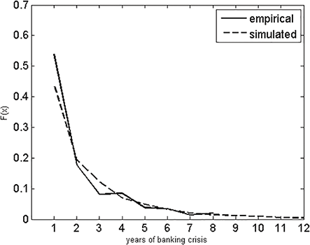
Figure 6 Distribution of banking crisis duration; simulated vs. empirical data. The length of a banking crisis is defined as the number of consecutive years with at least one banking failure in the country (Reinhart & Rogoff, Reference Reinhart and Rogoff2009).
The micro foundation of the labour market structure and dynamics further enriches the list of empirical regularities matched by the model and also debunks the robustness of some other ‘stylised facts’. More specifically, the extended K+S model is able to account for (roughly) the Beveridge curve (i.e. the negative correlation between unemployment and vacancy rates; see Figure 7 showing patterns as rough as the real ones), the Matching function (the positive correlation between vacancy-to-unemployment and job-finding rates; see Figure 8), the Wage curve, and the Okun curve (SF11-14; see Dosi et al., Reference Dosi, Pereira, Roventini and Virgillito2017, also for a detailed discussion of the other stylised facts). The model also replicates the analysis performed in Shimer (Reference Shimer2005) concerning the correlation structure between unemployment, vacancy, job finding, separation, and productivity (SF15; see Table 4). On the debunking side, the results from our model add doubts on the robustness of the ‘Phillips curves’ (as already discussed by Solow, Reference Solow1990; see also the recent Ratner & Sim, Reference Ratner and Sim2022), which might indeed be conditional on specific periods and institutional regimes.
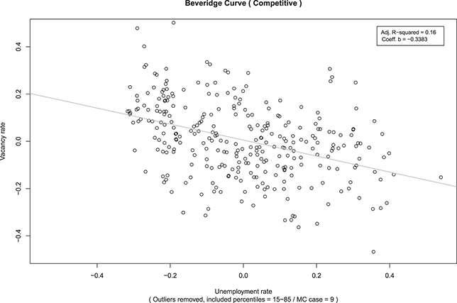
Figure 7 Beveridge curve (Dosi et al., Reference Dosi, Pereira, Roventini and Virgillito2017).
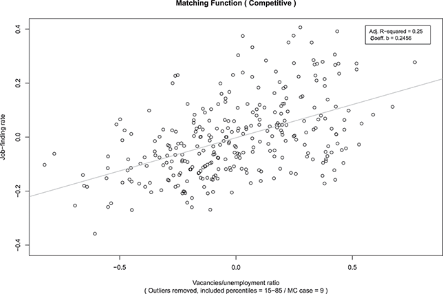
Figure 8 Matching function (Dosi et al., Reference Dosi, Pereira, Roventini and Virgillito2017).
Table 4 Correlation structure for Shimer (Reference Shimer2005) statistics;
unemployment,
vacancy,
job finding,
separation,
productivity.


| u | v | v/u | f | s | p | |
|---|---|---|---|---|---|---|
| Std. dev. | 0.05 | 0.234 | 0.266 | 0.152 | 0.153 | 0.051 |
| Autocorrelation | 0.56 | 0.604 | 0.613 | 0.476 | 0.467 | 0.888 |
| u | 1.00 | −0.612 | −0.718 | 0.488 | 0.602 | 0.130 |
| v | 1.000 | 0.990 | −0.532 | −0.612 | 0.084 | |
| v/u | 1.000 | −0.555 | −0.647 | 0.050 | ||
| f | 1.000 | 0.968 | −0.068 | |||
| s | 1.000 | −0.050 | ||||
| p | 1.000 |
6.2 Microeconomic Empirical Regularities
Beyond accounting for macroeconomic stylised facts, the family of the Schumpeter meeting Keynes models is also able to match the rather long list of microeconomic empirical regularities reported in Table 2.
Let us first consider those concerning the cross-sectional dynamics of firms (Bartelsman & Doms, Reference Bartelsman and Doms2000; Dosi, Reference Dosi, Malerba and Brusoni2007). Rank-size plots and normality tests suggest that cross-section firm (log) size distributions are skewed and not log-normal (SF16; see Figures 9 and 10 and Table 5). Moreover, firm growth-rate distributions are ‘tent-shaped’ (SF17; see Table 6) with tails fatter than the Gaussian benchmark (Table 6; see Bottazzi & Secchi, Reference Bottazzi and Secchi2003, Reference Bottazzi and Secchi2006).
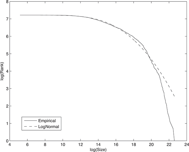
Figure 9 Pooled (year-standardised) capital-good firm sales distributions. Log rank vs. log size plots.
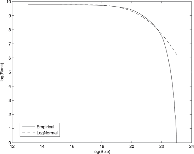
Figure 10 Pooled (year-standardised) consumption-good firm sales distributions. Log rank vs. log size plots.
Table 5 Log-size distributions, normality tests.
| Industry | Jarque–Bera | Lilliefors | Anderson–Darling | |||
|---|---|---|---|---|---|---|
| stat. | p-value | stat. | p-value | stat. | p-value | |
| Capital-good | 20.7982 | 0 | 0.0464 | 0 | 4.4282 | 0 |
| Consumption-good | 3129.7817 | 0 | 0.0670 | 0 | 191.0805 | 0 |
Table 6 Growth-rate distributions, estimation of exponential-power parameters.
| Series | b | Std. Dev. | a | Std. Dev. | m | Std. Dev. |
|---|---|---|---|---|---|---|
| Capital-good | 0.5285 | 0.0024 | 0.4410 | 0.0189 | −0.0089 | 0.0002 |
| Consumption-good | 0.4249 | 0.0051 | 0.0289 | 0.0037 | −0.0225 | 0.0001 |
Turning to firm productivity, again in line with the empirical evidence (Bartelsman & Doms, Reference Bartelsman and Doms2000; Dosi, Reference Dosi, Malerba and Brusoni2007), firms strikingly differ in terms of labour productivity (SF18; compare the standard deviations of labour productivity across firms plotted in Figure 11). Moreover, such productivity differentials persist over time (SF19; see the firm productivity autocorrelations reported in Table 7).Footnote 52

Figure 11 Firms’ Productivity Moments (logs). First panel: capital-good firms. Second panel: consumption-good firms.
Table 7 Average autocorrelation of productivity. Standard deviations in parentheses.
| Industry | t–1 | t–2 |
|---|---|---|
| Capital-good | 0.5433 | 0.3700 |
| (0.1821) | (0.2140) | |
| Consumption-good | 0.5974 | 0.3465 |
| (0.2407) | (0.2535) |
The model is also able to generate as an emergent property investment lumpiness SF20; see Doms & Dunne, Reference Doms and Dunne1998; Caballero, Reference Caballero, Taylor and Woodford1999). Indeed, in each time step, consumption-good firms with ‘near’ zero investment coexist with firms experiencing investment spikes (see Figure 12 and relate it to Gourio & Kashyap, Reference Gourio and Kashyap2007).

Figure 12 Investment lumpiness. First panel: share of firms with (near) zero investment; second panel: share of firms with investment spikes.
New microeconomic stylised facts are matched when heterogenous banks and workers are added to the K+S model. Firms’ bankruptcies are counter-cyclical (SF21, see Jaimovich & Floetotto, Reference Jaimovich and Floetotto2008), and the distribution of firms’ bad debt at bankruptcy follows a power law (SF22), in tune with the empirical evidence (Di Guilmi et al., Reference Di Guilmi, Gallegati and Ormerod2004). Finally, the labour-augmented K+S model replicates fat-tailed unemployment time distribution, fat-tailed wage growth rates distributions, and heterogenous worker-skill distributions (SF23–25).
7 Policy Experiments
Given the extremely good interpretative performance of the Keynes meeting Schumpeter family of models, let us employ it to assess the short- and long-run impact of different policies.Footnote 53 In particular, we study the impact of changes in either the parameter values or the policy scenarios on the GDP and productivity growth rates, the ratio of public debt to GDP, output volatility, and the unemployment rate. We consider here policies affecting the two main sources of economic change, namely innovation (see Section 7.1) and demand (see Section 7.2), that is, the ‘Schumpeterian’ and ‘Keynesian’ engines of growth. Finally, we consider the relationship between income distribution and the effectiveness of policies (see Section 7.3). The full list of experiments is discussed in Dosi, Fagiolo & Roventini (Reference Dosi, Fagiolo and Roventini2010); Dosi et al. (Reference Dosi, Fagiolo, Napoletano and Roventini2013, Reference Dosi, Fagiolo, Napoletano, Roventini and Treibich2015, Reference Dosi, Pereira, Roventini and Virgillito2017, Reference Dosi, Pereira, Roventini and Virgillito2018a, Reference Dosi, Pereira, Roventini and Virgillito2019, Reference Dosi, Freeman, Pereira, Roventini and Virgillito2021). The corresponding parameter values are spelled out in Table A.3 in Appendix A.
7.1 Tuning the Schumpeterian Engine: Innovation Policy Matters
We start by considering how technology policies concerning firm search capabilities and technological opportunities affect the long-run performance of the economy and also its short-run dynamics (Section 7.1.1). Then we study a set of policies targeting appropriability conditions and the industrial dynamics of the economy (entry and competition; see Section 7.1.2).Footnote 54
7.1.1 Technology Policies
Here we focus upon the ‘Schumpeterian side’ of the economy, holding the ‘Keynesian engine’ constant as compared with the benchmark scenario: Table 8 summarises the results. Let us start by turning off endogenous technological opportunities. In this case, the model collapses into a barebones 2-sector Solow (Reference Solow1956) model in steady state, with fixed coefficients and zero growth (absent demographic changes).
Table 8 Technology policy experiments. Normalised values compared to the benchmark across experiments, for 100 simulation runs. Absolute value of the simulation
-statistic in parentheses; (**) significant at 5 level, (*) significant at 10 level.

| Experiment | E1 Search capabilities | E2 Technological opportunities | ||
|---|---|---|---|---|
| low | high | low | high | |
| GDP growth | 0.917** | 1.063** | 0.774** | 1.250** |
| (7.425) | (5.657) | (25.491) | (22.274) | |
| GDP volatility | 1.020 | 0.958** | 0.981 | 1.023* |
| (1.505) | (3.198) | (1.411) | (1.919) | |
| Unemployment rate | 1.097 | 0.962 | 1.266** | 0.956 |
| (1.345) | (0.592) | (4.031) | (0.658) | |
In the first experiment, we change firm search capabilities (E1) approximated by the probabilities of accessing ‘innovations’ – no matter if failed or successful ones – (see the
 parameters in Eqs. 4 and 5). We find that higher search capabilities positively influence the GDP rates of growth, while lowering the unemployment (see Table 8). Together, business cycle fluctuations are dampened possibly because a population of ‘more competent’ firms entails lower degrees of technological asymmetries across them and indeed also lower degrees of ‘creative destruction’, with more ‘creative accumulation’ of innovative capabilities.
What happens if one varies the technological opportunities of innovation and the ability to search for them? The second experiment (E2, see Table 8) explores such a case. As compared to the benchmark, we shift rightward and leftward the mass of the Beta distribution governing new technological draws (i.e. the parameters
 and
and
 ; see Section 5.2). Note that the support of the distribution remains unchanged, so that one could informally state that the notional possibilities of drift in the technological frontier remain unchanged, too. However, the pool of opportunities agents actually face gets either richer or more rarefied. As one could expect, we find that higher opportunities have a positive impact on the long-term rate of growth. Such policies also reduce the average unemployment, while slightly increasing GDP volatility (a mark of Schumpeterian ‘gales of creative destruction’?).
7.1.2 Industrial Policies
The second set of experiments concerns the impact of policies affecting appropriability conditions and industry dynamics (experiments E3–E6 in Table 9).
Table 9 Industrial policy experiments. Normalised values compared to the benchmark across experiments, for 100 simulation runs. Absolute value of the simulation t-statistic in parentheses; (**) significant at 5% level, (*) significant at 10% level.
| Experiment | E3 Patents | E4 Entrant expected prod. | E5 Market selection | E6 Antitrust | ||||
|---|---|---|---|---|---|---|---|---|
| length | breadth | low | high | weak | strong | weak | strong | |
| GDP growth | 0.960** | 0.647** | 0.726** | 1.492** | 1.000 | 0.992 | 1.052** | 1.083** |
| (3.536) | (39.802) | (19.137) | (43.841) | (0.000) | (0.707) | (4.596) | (9.391) | |
| GDP volatility | 0.941** | 0.780** | 0.986 | 0.862** | 1.038** | 0.933** | 0.863** | 0.628** |
| (4.515) | (17.981) | (0.792) | (12.148) | (2.916) | (5.857) | (12.040) | (94.626) | |
| Unemployment rate | 1.056 | 1.240** | 1.308** | 0.796** | 1.169** | 0.955 | 0.966 | 0.781** |
| (0.768) | (3.074) | (3.376) | (3.191) | (2.364) | (0.659) | (0.546) | (3.814) | |
A tricky but relevant issue – both from the interpretative and normative points of view – regards the role of appropriability conditions (and, in particular, patents) as an incentive or an obstacle to innovation. The notion that some departure from the competitive zero profit condition is necessary in order to motivate capitalists to undertake search with their own money is at the core of the Schumpeterian (but also, earlier, Marxian) view of endogenous innovation. But how big should be such a departure? Neo-Schumpeterian models, as known, tend to assume monotonicity between degrees of appropriability and intensity of search, and, thus, rates of innovation (Aghion & Howitt, Reference Aghion and Howitt1992). The assumption, other things equal, in turn rests upon some form of ‘rational technological expectations’. Conversely, evolutionary models abhor the latter and assume much more routinized search behaviours. Recently, a large body of theoretical and empirical literature (see e.g. the contributions of Cimoli et al., Reference Cimoli, Dosi, Maskus, Okediji, Reichman and Stiglitz2014 and Dosi et al., Reference Dosi, Palagi, Roventini and Russo2022) have suggested that stricter property rights could be detrimental to innovation and growth. We exploit the modularity and flexibility of our agent-based model and introduce a patent system. More specifically, we test two alternative hypotheses (E3): in the ‘length only’ patent scenario, firms cannot imitate new technologies for a fixed number of periods; in the ‘breadth’ patent regime, firms are also forbidden to innovate around newly discovered technologies. We find that patents are detrimental both to long-run growth and to the short-run performance of the economy, being conducive to persistently higher unemployment rates (see Table 9). The negative impact of patents is stronger in the ‘breadth’ regime.Footnote 55
We then test the effects of firm entry on competition and innovation by changing entrants’ expected productivity (E4). We know empirically that most entrants are failures, but some are carriers of novel and potentially radical techniques and products (Dosi et al., Reference Dosi, Malerba, Marsili and Orsenigo1997; Bellone et al., Reference Bellone, Musso, Nesta and Quéré2008; Aghion et al., Reference Aghion, Blundell, Griffith, Howitt and Prantl2009). This is sometimes dramatised in the evolutionary literature as a ‘Schumpeterian Mark I’ versus a ‘Schumpeterian Mark II’ scenario, meaning systematic innovative advantages for entrepreneurial entrants versus cumulative advantages of incumbents (see Dosi et al., Reference Dosi, Marsili, Orsenigo and Salvatore1995; Malerba & Orsenigo, Reference Malerba and Orsenigo1995). How important are successful entrants? That is, from the normative point of view, what is the impact of policies favouring the entry of new competent firms? In our model, technological entry barriers (or advantages) are captured by the probability distribution over the ‘technological draws’ of entrants. Again, we hold constant the support over which the economy (i.e., every firm thereof) may draw innovative advances, conditional on the technology at any
 . In this case we do it for sake of consistency: results, even more so, apply if different regimes also entail different probability supports. Let us first tune the Beta distribution parameters
 and
and
 (see Section 5.4). Our results are broadly in line with the evidence discussed in Aghion and Howitt (Reference Aghion and Howitt2007): other things being equal, the easiness of entry and competence of entrants bear a positive impact upon long-term growth, mitigate business cycle fluctuations, and reduce average unemployment (see Table 9). However, the ceteris paribus condition is equally important: the same aggregate growth patterns can be proved to be equally guaranteed by competent cumulative learning of incumbents (see the earlier exercises on search capabilities).
Finally, we explore the effect of competition (and relatedly, competition policies) by altering market selection in the consumption-good industry (E5) and by introducing antitrust policies in the capital-good sector (E6). An idea broadly shared across the economic discipline is that ‘more competition is generally good’. In our model, that translates somewhat narrowly into a less imperfect access to information on prices by multiple heterogenous customers. In this case, in principle quite similar to the formally slimmer Phelps and Winter (Reference Phelps, Winter and Phelps1970), higher competition is reflected by the higher replicator dynamics parameter
 in Eq. 14. Simulation results suggest that a fiercer competition has negligible effects on growth, while it appears to somewhat reduce output volatility and average unemployment (see E5 in Table 9). We then introduce antitrust policies by limiting the maximum market share of capital-goods firms to 75% (weak case) or 50% (strong case). The outcome of this policy experiment is a lower unemployment rate, smaller business cycle fluctuations and also higher GDP growth (see E6 in Table 9; on this point see also Fogel, Morck, & Yeung, Reference Fogel, Morck and Yeung2008). Note that such a property have little to do with any static ‘welfare gains’ – which our model does not explicitly contemplate – but rather with the multiplicity of producers, and thus of innovative search avenues, which antitrust policies safeguard.Footnote 56
7.2 Necessity of Keynesian Policies: Demand and Institutions Matter
So far, we have explored the effects of different ‘Schumpeterian’ policies and organisational set-ups over, for example, the rate of growth of the economy, the unemployment rates, and so on. The above sets of experiments clearly indicate that the sources of growth in the model lie in firms’ ability to search efficiently and to develop improved products and processes, significantly affecting also the short-run dynamics of the economy. However, to repeat, such results are conditional on a ‘Keynesian machine’ well in place. What happens if we switch that off?
A first rough but very robust answer comes from the comparison between the foregoing regime with a set-up whereby all ‘Keynesian’ policies are turned off and the system lives under a ‘pure Schumpeterian regime’, holding, however, constant technological opportunities, search rules, and competition dynamics, as in the benchmark model (E7; see also Dosi, Fagiolo, & Roventini, Reference Dosi, Fagiolo and Roventini2010). Turning off the ‘Keynesian’ component implies a major jump to a different phase of the system, characterised by nearly zero growth and enormous fluctuations (see Table 10, column 2). This is because, by sustaining demand during recessions, countercyclical Keynesian policies also smooth investment over the business cycle. Low demand indeed reduces both consumption-goods firms’ investment and capital-goods firms’ R&D expenses, thus rates of innovation and productivity growth. Such a vicious circle of low R&D, low economic growth, and high volatility is in line with previous accounts by Stiglitz (Reference Stiglitz, Shionoya and Perlman1994) and Aghion et al. (Reference Aghion, Askenazy, Berman, Cette and Eymard2008) and Aghion et al. (Reference Aghion, Angeletos, Banerjee and Manova2010), in particular in the presence of credit market imperfections (Aghion, Hemous, & Kharroubi, Reference Aghion, Hemous and Kharroubi2014).
Table 10 Keynesian policy experiments. The ‘strong’ Schumpeterian regime is set with high technological opportunities and high search capabilities. Normalised values compared to the benchmark across experiments, for 100 simulation runs. Absolute value of the
-statistic in parentheses; (**) significant at 5 level, (*) significant at 10 level.

| Experiment | E7 Schumpeterian regime | E8 Stabilisers | |||
|---|---|---|---|---|---|
| pure | strong | weak | strong | very strong | |
| Subsidy rate | 0 | 0 | 0.2 | 0.6 | 0.8 |
| Tax rate | 0 | 0 | 0.05 | 0.15 | 0.2 |
| GDP growth | 0.139** | 0.437** | 1.008 | 0.996 | 1.008 |
| (17.837) | (7.841) | (0.707) | (0.354) | (0.707) | |
| GDP volatility | 19.611** | 19.173** | 1.902** | 0.779** | 0.722** |
| (47.186) | (34.426) | (28.119) | (20.808) | (24.405) | |
| Unemployment | 10.962** | 7.327** | 2.413** | 0.789** | 0.562** |
| rate | (37.639) | (24.353) | (8.846) | (3.738) | (8.271) |
The experiments discussed earlier indicate that Schumpeterian and Keynesian policies affect, together, short-term economic indicators (e.g., output volatility and employment), as well as long-term ones (e.g., GDP growth). Still, these experiments were implemented considering ‘everything else being equal’: an active technology policy was tested, taking as fixed the fiscal side of the model, and the other way round. Could technology policies be a substitute for a lack of fiscal policies? We test this proposition by experimenting with a ‘strong Schumpeterian regime’ (high search capabilities and technological opportunities) combined with a zero fiscal policy scenario (no taxes and unemployment subsidies). Table 10 (column 3) shows that in this case average GDP growth falls by 56% with respect to the baseline. Notice that it is exactly the net effect from both policies. Indeed, the former increases the average GDP growth rate (respectively, by 6% and 25%), while the latter has a negative impact amounting to a 86% cut in the long-run rate of output growth. It follows that Keynesian policies are complementary to Schumpeterian ones, as the latter alone cannot sustain a stable growth path.
In the K+S benchmark model, taxes and unemployment subsidies act as automatic stabilisers, dampening business cycle fluctuations. In experiment E8 (Dosi et al., Reference Dosi, Fagiolo and Roventini2010), we jointly modify the intensity of these stabilisers by altering the tax and subsidy rates
 and
and
 (see Section 5.6). Results in Table 10 show the impact of Keynesian fiscal policies upon long-run economic growth and short-run dynamics. In the presence of the ‘good phase’ of the system (to repeat, with positive tax and subsidy; see Figure 13), higher levels of automatic stabilisers do not affect average GDP, but they further stabilise output fluctuations: GDP volatility and unemployment rates fall as taxes and subsidy rates are jointly increased.Footnote 57
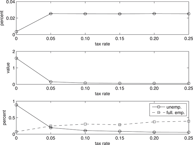
Figure 13 Fiscal policy experiments (Dosi, Fagiolo, & Roventini, Reference Dosi, Fagiolo and Roventini2010). First panel: average output growth rate. Second panel: bandpass-filtered output standard deviation. Third panel: average unemployment rate (unemp.) and full-employment frequency (full emp.). In such policy experiments, the unemployment subsidy rate (
 ) is four times the tax rate.
7.2.1 Fiscal Austerity Rules
Let us now further test the impact of Keynesian fiscal policies by studying the impact of different austerity fiscal rules akin to those implemented in the European Union. We first consider a fiscal rule mimicking the European Stability and Growth Pact (SGP; see Dosi et al., Reference Dosi, Fagiolo, Napoletano, Roventini and Treibich2015) which constrains the public deficit to 3% of GDP, forcing the government to cut unemployment subsidies until the deficit-to-GDP target is reached. We then introduce the stricter Fiscal Compact (FC) rule, where the the SGP deficit limit is supplemented by a debt-reduction rule: if the ratio of public debt to GDP is over the SGP target of 60%, it should be reduced by 1/ 20th (5%) of the difference between the current and target levels in every year.Footnote 58 In both regimes, unemployment benefits are eventually cut to comply with the fiscal rules. In line with the European Union fiscal framework, we introduce escape clauses (
 and
and
 ) which freeze austerity rules in case of negative GDP growth. Finally, we account for the possible existence of a positive feedback mechanism going from the level of public debt to its financing cost by adding a risk premium to the interest rate on sovereign bonds. In such a scenario with the FC fiscal rule (
 ), ‘frugal’ governments should pay a lower interest rate on their stock of public debt.
The results from the fiscal rule experiments (E9; see Table 11) point, again, to the necessity of active fiscal policy to stabilise the economy and achieve steady growth. Indeed, we find that in the ‘harsh’ case, when the
 fiscal rule is applied, average GDP growth is halved compared to the baseline scenario, and GDP volatility and unemployment are respectively 14 and 5 times higher. Moreover, the public-debt-to-GDP ratio explodes due to the joint expansion of debt and the shrinkage of output, showing the self-defeating effect of fiscal discipline policies. The negative impact of austerity fiscal rules is even more harmful in the Fiscal Compact scenario. When escape clauses are present (
 e
e
 ), the long-run harmful effects of fiscal discipline disappear, but volatility and unemployment rates are still significantly higher with respect to the case where fiscal policy is unconstrained (see Table 10). These findings shed light on the non-linear effects of fiscal policies on GDP growth (see Figure 13), as the halt to fiscal support during recessions is likely to transform them in depressions. Finally, the results are also robust when the spread on sovereign bonds is linked to the ratio between public debt and GDP (
 ): austerity rules worsen both short- and long-run economic dynamics without improving public finances.Footnote 59
Table 11 Fiscal policy experiments. Normalised values compared to the benchmark across experiments, for 100 simulation runs. Absolute value of the
-statistic in parentheses; (**) significant at 5 level, (*) significant at 10 level.

| Experiment | E9 | ||||
|---|---|---|---|---|---|
| SGP |

| FC |

|

| |
| GDP growth | 0.527** | 0.995** | 0.572** | 0.992** | 0.997** |
| (6.894) | (0.876) | (6.499) | (1.388) | (0.524) | |
| GDP volatility | 14.645** | 1.408** | 16.204** | 1.624** | 1.530** |
| (7.466) | (5.856) | (7.848) | (7.166) | (6.962) | |
| Unemployment | 5.692** | 5.706** | 1.419 | 1.948** | 1.679** |
| rate | (8.095) | (2.088) | (7.585) | (3.928) | (3.139) |
| Public Debt/GDP |

| 1.763** |

| 4.078** | 2.590** |
| (0.774) | (2.472) | (1.483) | |||
One of the advantages of employing agent-based models to study economic problems is the possibility of zooming upon the microeconomic level to better understand the emergent properties observed at the macro level. The wealth of microeconomic data generated by the simulations can indeed be employed to build new statistics which can shed light on macroeconomic dynamics. This is what we do with the microeconomic indicators displayed in Table 12, which allow us to study the underlying micro-level mechanisms at the origin of the aggregate outcomes observed when fiscal rules are in place (see Dosi et al., 2016). First, we consider the consumption-good sector. We find that firms’ investment rate falls due to the lower consumption demand. This slows down the diffusion of the new vintages of machines with state-of-the-art technology thus depressing productivity growth. The negative impact of austerity policies percolates to the capital-good sector. There, the lower sales experienced by capital-good firms reduce their R&D investment. As a result, innovation falls, slowing down the productivity growth of the industry (see Table 12). The reduced creation and diffusion of innovations imply that the best vintage stays undisputed for a longer period, and the productivity frontier grows at a slower pace. Indeed, this represents a power evidence of the (virtuous or perverse) feedback between the ‘Keynesian’ demand-generating mechanism and the long-term movement of the technological frontier.
Table 12 Fiscal rule – microeconomic indicators. Normalised values compared to the benchmark across experiments, for 100 simulation runs. Absolute value of the
-statistic in parentheses; (**) significant at 5 level, (*) significant at 10 level.

| Experiment | E9 Fiscal rule SGP | |
|---|---|---|
| Innovation creation in the capital-good sector | ||
| Share of successful innovators | 0.946** | (2.762) |
| Productivity growth | 0.980** | (2.269) |
| Productivity dispersion | 0.917** | (6.538) |
| Innovation diffusion in the consumption-goods sector | ||
| Productivity growth | 0.889** | (3.912) |
| Productivity dispersion | 0.865** | (3.429) |
| Investment rate | 0.973 | (1.275) |
| Duration of best vintage | 1.037** | (3.927) |
| Productivity growth best vintage | 0.954** | (34.446) |
| Relative distance between | 0.970** | (2.432) |
| best and worst vintages | ||
7.2.2 Labour Market Reforms
In contrast to DSGE models, macroeconomic agent-based models can easily test different combinations of policies concerning the labour and credit markets. We undertake two sets of policy experiments. In the first one, we study the interactions between fiscal policies and different labour-market institutions governing wage formation, firm firing rules, etc. (E10). In the next section, we will present the second policy combination scenario, where we interact fiscal policies with monetary policy rules (E11).
How do labour market institutions affect the short- and long-run performance of the economy and interact with fiscal policy rules? In the ‘Fordist’ regime, the labour-augmented K+S model presented in Section 5.8 depicts a scenario where (i) wages are insensitive to the labour-market conditions and indexed to aggregate and firm-specific gains; (ii) there is a sort of covenant between firms and workers concerning ‘long-term’ employment, as firms fire only when their profits get negative, while employed workers do not seek for alternative occupations; (iii) labour market institutions contemplate a minimum wage fully indexed to aggregated economy productivity and unemployment benefits financed by taxes on profits. The ‘Fordist’ regime captures the main features of the Trente Glorieuses (roughly the three decades after World War II) characterised by low probability of workers being fired, wage dynamics mostly rigid to the business cycle, wage growth rate indexed upon productivity growth, a shrinking degree of inequality, and significant, tax-based unemployment benefits.
At the opposite end when the labour market is characterised by the ‘Competitive’ regime, (i) flexible wages respond to unemployment and market conditions; (ii) firms have a stronger bargaining power with regard to wages and employment, which they seamlessly adjust according to the planned production level; (iii) employed workers search for better paid jobs; (iv) the minimum wage and unemployment benefit institutions are weaker or even absent. The Competitive scenario is akin to the labour market presented in introductory-level Neoclassical economics textbooks and it captures the structural reforms suggested by the Washington Consensus and the European Union (Fitoussi & Saraceno, 2013).
We simulate the model in the Fordist and Competitive regimes (see Table 13). Simulation results show that labour market flexibility worsens the performance of the economy both over short- and long-run horizons. Indeed, the unemployment rate is higher in the Competitive regime, while the Fordist regime entails stronger productivity and output growth. Note that the degradation of economic performance increases with the degree of labour-market flexibility: in Dosi et al. (Reference Dosi, Pereira, Roventini and Virgillito2017) we find that in the Competitive scenario nearest to ‘market perfection’ (absence of minimum wage, unemployment benefits, and employment protection rules), the modelled economic system is most of the time near to collapse with basically zero long-term economic growth and extremely high unemployment rates and volatility. This result is in line with those obtained earlier when the Keynesian machine is switched off. Moreover, we find that hysteresis is much more likely to emerge in the Competitive regime, thus worsening macroeconomic dynamics at all frequencies (see Figure 14 and the results in Dosi et al., Reference Dosi, Pereira, Roventini and Virgillito2018a).
Table 13 Labour-market reform experiments. Normalised values compared to the benchmark across experiments, for 50 simulation runs. P-values in parentheses; (**) significant at 5 level, (*) significant at 10 level.
| Experiment | E10 | ||
|---|---|---|---|
| Fordist (baseline) | Competitive (ratio) | Competitive & Fiscal Compact (ratio) | |
| GDP growth | 0.02 | 0.78** | 0.68** |
| (0.01) | (0.00) | ||
| GDP volatility | 0.11 | 0.86** | 1.19** |
| (0.01) | (0.00) | ||
| Unemployment rate | 0.02 | 8.93** | 10.96** |
| (0.00) | (0.00) | ||
| Profit share | 0.22 | 1.02** | 1.03** |
| (0.00) | (0.00) | ||
| Income concentration | 0.05 | 3.60** | 5.09** |
| (0.00) | (0.00) | ||

Figure 14 GDP long-term trend recovery after crisis (Dosi et al., Reference Dosi, Pereira, Roventini and Virgillito2019). Typical simulation run. Top: Fordist; middle: Competitive; bottom: Competitive and Fiscal Compact rule. Dashed line: pre-crisis trend | grey boxes: trend recovery period.
The negative impact of the Fiscal Compact rule is magnified when the labour market is characterised by a higher level of flexibility (see Table 13).Footnote 60 Indeed, the policy combination of austerity rule and competitive labour-market reforms permanently damage the GDP growth trajectory and spur unemployment, leading to the emergence of super-hysteresis (see Figure 14; Dosi et al., Reference Dosi, Pereira, Roventini and Virgillito2018a and Cerra et al., Reference Cerra, Fatás and Saxena2023). Also in this case austerity policies are self-defeating, leading to higher levels of public debt (see the detailed analysis in Dosi et al., Reference Dosi, Pereira, Roventini and Virgillito2019). To sum up, our results clearly show that the policy combination grounded on ‘structural reforms’ to increase labour flexibility and austerity fiscal policies (the so called Berlin–Washington consensus; see Fitoussi & Saraceno, Reference Fitoussi and Saraceno2013) have a deeply negative impact on the short- and long-run performance of the economy, and also on public finances.
7.2.3 Monetary Policy
In the foregoing experiments, the central bank followed a ‘conservative’ monetary policy as it applied a standard Taylor rule which adjusts the baseline interest rate only to the inflation gap (
 ; see Eq. 18). In line with the recent monetary policy strategy of the Federal Reserve (Yellen, Reference Yellen2014), we now let the central bank follow a dual-mandate monetary policy (
 ) by including an adjustment to the unemployment gap (
 ), with a 5% unemployment rate target (E11).
Simulation results reported in Table 14 show that when fiscal policy is unconstrained and the central bank commits to both price and employment stabilisation, monetary policy positively affects the performance of the economy. When the SGP fiscal rule is activated, the positive impact of the dual-mandate monetary policy is reinforced, as it contributes to alleviate the pains caused by fiscal-consolidation policies and to stabilise public finance. The dual-mandate Taylor rule dominates the conservative one also in the presence of the FC rule, when fiscal clauses are activated and when the bond-spread channel is taken into account.Footnote 61
Table 14 Monetary policy experiments. Normalised values compared to the benchmark across experiments, for 100 simulation runs. Absolute value of the
-statistic in parentheses; (**) significant at 5 level, (*) significant at 10 level.

| Experiment | E11 | ||
|---|---|---|---|

|

|

| |
| GDP growth | 1.019** | 0.527** | 1.014 |
| (3.730) | (6.894) | (1.157) | |
| GDP volatility | 0.865** | 14.645** | 2.760** |
| (6.018) | (7.466) | (2.401) | |
| Unemployment rate | 0.322** | 5.692** | 0.909 |
| (5.903) | (8.095) | (0.555) | |
| Public Debt/GDP | −50.648** |

| −45.545** |
| (30.377) | (9.011) | ||
The better performance of the
 rule over the
 depends on the presence of bank credit transmission channels of monetary policy (see e.g. Bernanke, Gertler, & Gilchrist, Reference Bernanke, Gertler, Gilchrist, Taylor and Woodford1999 and Boivin, Kiley, & Mishkin, Reference Boivin, Kiley, Mishkin, Friedman and Woodford2010) due to the interaction of the dual-mandate monetary policy with the Basel rule governing changes in credit supply (see Eq. 17). By reducing the pro-cyclicality of the Basel macroprudential rule, the dual mandate therefore compensates its destabilising effect and provides both banks and firms with a stronger financial record at the eve of an economic crisis. Indeed, with a dual-mandate monetary policy rule, the interest rate goes up during expansions as a response to low unemployment levels. This boosts banks’ profit margin and net worth, while cooling down firms’ borrowing. When the downturn arrives, the interest rate goes down and loan losses increase. However, banks’ capital buffers allow them to better resist the negative shocks and provide more credit vis-à-vis the conservative Taylor rule scenario.
7.3 Income Inequality and Policy Effectiveness: Distribution Matters
In macro agent-based models, policy experiments can be performed in alternative scenarios concerning the structural and institutional characteristics of the economy, as well as with respect to personal and functional income distributions. Admittedly, all the incumbent K+S models are constrained by the assumption of initial levels of mark-ups of the firm which partly ‘anchor’ the average functional income distribution thereafter. This indeed is a drawback to be overcome in the near future. Still, even under this limitation, it is highly informative to study the impact of alternative combination of policies on the level of functional income inequality in the economy (E12), and, even more so, on the personal distribution with respect to wage earners.
The policy experiments performed so far have been carried out for a given level of income inequality. Indeed, the firm-specific mark-ups of consumption-good firms fluctuate around the initial peg; see Eqs. 11 and 12. By tuning up and down the level of the initial mark-up rate, we can (admittedly, still in a rudimentary way) change the long-term functional income distribution. This allows us to study how inequality affects the dynamics of the economy, as well as the results produced by the different mixes of policies spotlighted in the previous section. In Dosi et al. (Reference Dosi, Fagiolo, Napoletano and Roventini2013), we found that a higher level of inequality in the wage/profit distribution increases the effects of fiscal policies. This is in line with many works suggesting that increasing levels of inequality have contributed to depress aggregate demand and to weigh down private indebtedness, thus setting the stage for the Great Recession (Fitoussi & Saraceno, Reference Fitoussi and Saraceno2010; Stiglitz, Reference Stiglitz2012; Kumhof & Rancière, Reference Kumhof and Rancière2015).
Given such premises, let us study how our target variables evolve when we modify the income distribution under the benchmark scenario where fiscal rules are not activated and the central bank follows a conservative Taylor rule. First, rising firm margins, reflected, of course, by higher income inequality, impact aggregate demand, and they thus affect macroeconomic dynamics (see Figure 15). If, on the one hand, the average GDP growth rate is stable for different levels of mark-up, on the other hand, the (slightly) U-shape pattern displayed by GDP volatility, unemployment rates, likelihood of economic crisis and public-debt-to-GDP ratio reveal the existence of two ‘regimes’. When mark-ups are low, firms have a reduced ability to finance their investment with their own accumulated profits and rely more on credit, increasing the size of banks and the cost of banking crises. Therefore the size of the banking sector is negatively associated with the mark-up rate. If mark-ups are too low, firms’ higher failure rates weaken the banking sector, thus curbing the supply of credit. As a consequence, a higher proportion of financially constrained firms reduces production and investment, leading to higher unemployment rates. When income distribution is too skewed towards profits, firms do not invest because demand is too low. This spurs GDP volatility, unemployment, and public debt (Dosi et al., Reference Dosi, Fagiolo, Napoletano and Roventini2013 and Reference Dosi, Fagiolo, Napoletano, Roventini and Treibich2015).

Figure 15 Income distribution and macroeconomic dynamics (Dosi et al., Reference Dosi, Fagiolo, Napoletano, Roventini and Treibich2015). Confidence-interval bands are shown in a lighter colour and are computed as plus or minus two Monte Carlo standard errors.
Let us now consider the impact of fiscal rules across different functional inequality scenarios. Income distribution and fiscal policies can interact via two channels. First, tighter limits on budget deficits can further depress aggregate demand, thus worsening firms’ financial constraints and increasing the likelihood of banking crises which require public bailout. Second, when the income distribution is more biased towards profits, fiscal policy is more needed to sustain an (otherwise low) consumption demand (see Dosi et al., Reference Dosi, Sodini and Virgillito2015). Simulation results show that for every level of functional income inequality, the SGP and FC fiscal rules increase the instability of the economy (see Figure 16) and inflate the ratio between public debt and GDP. Moreover, fiscal discipline appears to be more harmful as the income distribution becomes more biased towards profits. Indeed, even if in this regime firms have access to both internal and external financial resources, they do not invest for a lack of aggregate demand, which in turn reduces the average GDP growth rate and leads to the explosion of the public-debt-to-GDP ratio.Footnote 62 Further exercises suggest that when the escape clauses are in place, they prevent the activation of fiscal rules up to 40% of the periods (Figure 16, bottom right), thus reducing their negative impact on the dynamics of the economy. Nonetheless, in line with our previous results, the economy keeps on being more unstable and we keep observing a perverse effect of fiscal rules on public debt. Such results are also confirmed in the sovereign bond-spread adjustment scenario.
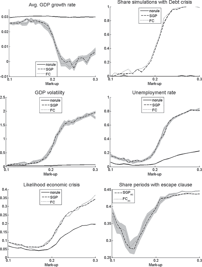
Figure 16 Fiscal rule experiments (Dosi et al., Reference Dosi, Fagiolo, Napoletano, Roventini and Treibich2015). Confidence-interval bands are shown in a lighter colour and are computed as plus or minus two Monte Carlo standard errors.
How does monetary policy interact with income inequality? In the presence of unconstrained fiscal policies, the dual-mandate Taylor rule outperforms the ‘conservative’ one for every level of inequality without leading to inflation spirals (see Figure 17). Which mechanisms are responsible for such dynamics? With a dual-mandate Taylor rule, the banking sector performs better, as the economy is characterised by a higher share of investment projects that are financed and implemented and a lower rate of banking failures. Lower unemployment pushes interest rates up, thus increasing banks’ profitability, while tightening firms’ constraints to invest. The increase of the interest rate cools down aggregate demand during booms, while improving the net worth of the banks, leading to a higher supply of credit when the economy experiences a downturn.

Figure 17 Monetary policy experiments (Dosi et al., Reference Dosi, Fagiolo, Napoletano, Roventini and Treibich2015). Confidence-interval bands are shown in a lighter colour and are computed as plus or minus two Monte Carlo standard errors.
Finally, the labour-augmented K+S model allows one to account for the evolution of both functional and personal inequality as heterogeneous workers can earn different wages. We find that the negative impact on economic dynamics of ‘structural reforms’ designed to increase the flexibility of the labour market reflects also in an increase of the profit share and in a higher personal income concentration (see Table 13). This is in line with the recent empirical evidence on the impact of policies to flexibilise the labour market (see, e.g., Hoffmann, Malacrino, & Pistaferri, Reference Hoffmann, Malacrino and Pistaferri2022; Daruich, Di Addario, & Saggio, Reference Daruich, Di Addario and Saggio2023). Not surprisingly, functional and personal inequalities further increase when fiscal austerity rules are applied to economies characterised by ‘Competitive’ labour markets.
7.4 Which Policies for Smooth Inclusive Growth?
The results presented in this section using the Schumpeter meeting Keynes models as a laboratory for simulation experiments illustrate how macreoeconomic agent-based models are a powerful and flexible tool for policy analysis. In particular, ABMs allow one to jointly test different ensembles of public interventions, for example innovation, industrial, fiscal and monetary policies, as well as market reforms. Moreover, the impact of policies can be studied at different frequencies, taking into account both their effect on business cycles and their influence on growth dynamics. Policy exercises can be conditioned to different institutional scenarios as shown by our experiments with alternative labour market regimes and different levels of income inequality. Naturally, actual decision makers can be effectively involved in the process of the design of macro agent-based models for policy evaluation (Moss, Reference Moss2008).
The results of the battery of policy exercises carried out with the K+S models exploit its capability to bridge Schumpeterian theories of technology-driven economic growth with Keynesian theories of demand generation. First, innovation and industrial policies affect both the long- and short-run performance of the economy. However, such policies tuning the ‘Schumpeterian engine’ are not sufficient to maintain the economy on a high-growth/near full-employment path. Indeed, the endogenous innovation engine is able to do that only in the presence of a ‘Keynesian’ demand-generating engine, which requires a policy mix comprising (i) an unconstrained fiscal policy, where automatic stabilisers are free to dampen business cycle fluctuations; (ii) a monetary policy targeting both price and employment stability; (iii) ‘rigid’ labour market institutions (strict firing rules, minimum wage, etc.). Such a policy combination is able to achieve lower unemployment and output volatility cum higher productivity and GDP growth.
More generally, our results dispose of the traditional dichotomy between variables impacting the long run (typically, ‘supply-side’ technology-related changes) and variables with a short-term effect (traditional demand-related variables). On the contrary, technological innovations appear to exert their effects at all frequencies. Conversely, Keynesian demand-management policies do not only contribute to reduce output volatility and unemployment rates, but they affect also long-run growth rates insofar as they contribute to ‘delock’ the economy from the stagnant growth trajectory, which is indeed one of the possible emergent meta-stable states linked to the structural characteristics of the economy such as functional income inequality. In that, the policy analysis exercises carried out with the K+S models are well in tune with the mentioned empirical evidence showing the ubiquitous presence of hysteresis in macroeconomic dynamics (Dosi et al., Reference Dosi, Pereira, Roventini and Virgillito2018a; Cerra et al., Reference Cerra, Fatás and Saxena2023).
8 A Brief Discussion on the Future of Macroeconomics by Way of a Conclusion
In a visionary note, Frank Hahn (Reference Hahn1991), indeed one of the founding fathers of General Equilibrium theory, was very pessimistic about current theorising in economics:
Thus we have seen economists abandoning attempts to understand the central question of our subject, namely: how do decentralized choices interact and perhaps get coordinated in favor of a theory according to which an economy is to be understood as the outcome of the maximization of a representative agent’s utility over an infinite future? Apart from purely theoretical objections it is clear that this sort of thing heralds the decadence of endeavor just as clearly as Trajan’s column heralded the decadence of Rome. It is the last twitch and gasp of a dying method. It rescues rational choice by ignoring every one of the questions pressing for attention.
But he indicates a route for economics for the next hundred years:
Instead of theorems we shall need simulations, instead of simple transparent axioms there looms the likelihood of psychological, sociological and historical postulates. ... In this respect the signs are that the subject will return to its Marshallian affinities to biology. Evolutionary theories are beginning to flourish, and they are not the sort of theories we have had hitherto. ... But wildly complex systems need simulating.
This moment is now. The Great Recession has prompted a debate about the state of macroeconomic theory, and standard DSGE models have been fiercely criticised by an increasing number of economists for their flaws, which, we believe, are so deep that they cannot be cured. At the same time, agent-based macroeconomics has blossomed naturally, accounting for all the economics problems that require heterogeneity and interactions, such as technical and structural change, inequality, financial intermediation, and so on.
This Element has shown how the Keynes meeting Schumpeter family of macro agent-based models is a credible alternative to discredited DSGE models. The K+S models are indeed able to pair Schumpeterian processes of innovation and creative destruction with Keynesian demand-coordination dynamics. In doing so, the approach is able to account for endogenous growth and business cycles punctuated by crises. Beyond accounting for such emergent properties, the K+S models are able to reproduce a rich list of macro and micro stylised facts. Different combinations of policies have been tested, revealing the strong profound complementarities between Schumpeterian innovation policies and Keynesian ones. The results produced by the K+S models unequivocally show the necessity of integrated macroeconomic models to fully grasp the evolution of capitalist economies, in line with the remarks of Solow (Reference Solow2005) and the recent empirical evidence on hysteresis (Cerra et al., Reference Cerra, Fatás and Saxena2023).
The generative potentiality of the family of Schumpeter meeting Keynes models – and more generally by macro agent-based models – is shown by the streams of recent works. Here are a few examples.
Concerning the very behavioural foundation, the impact on macroeconomic dynamics of different forms of heterogeneous and boundedly rational expectations is studied in Dosi et al. (Reference Dosi, Napoletano, Roventini, Stiglitz and Treibich2020a). Simulation results show that fast and frugal heuristics (Gigerenzer & Brighton, Reference Gigerenzer and Brighton2009) are ‘rational’ responses in complex evolving economies, outperforming OLS-leaning expectations which spur the instability of the system.
The family of K+S models has also expanded along three complementary directions.
In the first direction, we have begun to tackle one of the fundamental questions which have puzzled the economic discipline since at least Ricardo, namely, under what conditions the jab-generation effect of technical progress, – basically associated with the introduction of new products and of the price reduction of existing ones –, compensates the labour-shedding effects productivity enhancements (Dosi et al., Reference Dosi, Pereira, Roventini and Virgillito2022).
Second, we have begun to explore the impact of labour market institutions, and in particular the presence or absence of unions, upon the dynamics of wages, inequalities, and, more generally, the whole economy (Dosi et al., Reference Dosi, Freeman, Pereira, Roventini and Virgillito2021; Dosi et al., Reference Dosi, Pereira, Roventini and Virgillito2024).
In the third line of research, we have started studying the co-evolution of climate and economic dynamics. More specifically, we have expanded the K+S model: (i) introducing an energy sector populated by heterogenous green and dirty plants, (ii) accounting for greenhouse gas emissions of firms, and (iii) studying the impact of microeconomic climate shocks. With the new Dystopian Schumpeter meeting Keynes model (Lamperti et al., Reference Lamperti2018 and Reference Lamperti, Dosi, Napoletano, Roventini and Sapio2020), we find that, in the absence of any climate policy, the climate impacts have catastrophic effects on economic dynamics. Such shocks are magnified by the financial system (Lamperti et al., Reference Lamperti, Bosetti, Roventini and Tavoni2019). At the same time, command and control and green industrial policies are able to decarbonise the economy while preserving sustainable growth (Wieners et al., Reference Wieners, Lamperti, Dosi and Roventini2024).
And there are quite a few domains still awaiting to be addressed within this art form. Just to name a few: (i) open economies, and more generally, multi-countries and multi-industries set-ups with flows of goods and finance (see Dosi, Roventini, & Russo, Reference Dosi, Roventini and Russo2019, Reference Dosi, Roventini and Russo2020, for the first attempts); (ii) more sophisticated accounts for the (endogenous) dynamics of income distribution, and role of that in conflict among social groups and classes; (iii) opening up the ‘organisational blackbox’ and the dynamics therein. And there are many others.
A particularly challenging issue concerns the relationship between high-dimensional phenomenologically rich models like the K+S ones, and much simpler lower-dimensional models on the functional links between unemployment, income distribution, and capital accumulation (see also Dosi, Usula, & Virgillito, 2024) or models of ‘multiplier-accelerator’ of Keynesian flavour such as Pasinetti (Reference Pasinetti1974). Our conjecture is that the two genres may be highly complementary in that the latter can be instrumental in deriving analytical predictions (not forecasts!) from relatively simple functional hypotheses, while the former are crucial in exploring the domains of their applicability. In between lies a huge field for statistical analyses, both on actual historical data and simulated ones. The ‘Phillips curve’ mentioned earlier is a good case to illustrate the point. Under what institutional set-ups does it emerge, both in the real world and in the simulated one? And similar questions apply to other purported ‘laws of motion’ such as the ‘accelerator’, the ‘Verdoorn–Kaldor law’, and so on, as well as, of course, debunking pure figments of imagination such as the AS and AD curves.
Moreover, a lot more exploration is required of the policy side. So, as an example, Dosi et al. (Reference Dosi, Lamperti, Mazzucato, Napoletano and Roventini2023) assess with a K+S model different types of direct and indirect innovation policies, taking also into account their impact on the public debt. They find that all policies improve productivity and GDP growth, but the best outcomes are achieved by active discretionary state policies, which are also able to crowd-in private investment and have positive hysteresis effects on growth dynamics.
If the foregoing developments suggest that the Dark Age of macroeconomics (Krugman, Reference Krugman2011) is perhaps approaching its end, what prevents agent-based models from becoming the standard way of theorising in macroeconomics? There are some reasons that are theoretical and others that are ‘political’.
On the theory side, it is certainly true that, as the old adage goes, no matter how badly a theory performs, ‘you need a model to replace another one’. However, the alternative macros – indeed more than one! – are already here. What are then the stumbling blocks?
First, as we have been arguing, over roughly the last half a century economics has undergone a thorough ‘anthropomorphisation’ of models. Nowadays, having a ‘structural model’ at whatever level of observation entails deriving empirical properties from ‘first principles’, that is, from whatever is axiomatic on max (something) under some arbitrary constraints. This has trickled down to common language and has merged with a wider laissez-faire ideology. So, in everyday discourse, ‘markets are optimistic, or nervous, or worried ...’. It is a humanised version of the rational-expectation-based representative agent story, which normatively has far-reaching ideological implications on the predominance of ‘incentive’, which is well beyond this discussion.Footnote 63 Of course, fifty years ago and more, this was not at all the normative. So, for example, Bob Solow and Luigi Pasinetti were debating, often bitterly, on the dynamics of the relative factor intensities, with Bob S. making propositions on the sign of the change based on some property of the purported production function and Luigi P. questioning that very property. Neither one would have dreamed of nesting their argument on what either ‘Mr. Market’, or, even less so, ‘Dr. Doe’ would have done! In doing so, however, Solow (take him as the persona of the American reasonable Keynesian growth analyst) took too lightly the ‘microfoundation challenge’ and the problems stemming from aggregation and from the lack of micro–macro isophormism, while at the opposite extreme, Luigi P. (with many economists of genuinely ‘Classical’ inspiration) always rejected the very notion of microfoundations, exclusively focusing on laws of motion at the system level. The ABM perspective, proposed here, accepts the microfoundation challenge, but fully acknowledges the lack of isomorphism, More is different, and interactions naturally entail complexity and emergence. There is no hope of evincing ‘anthropomorphism’ at all costs, thus shrinking macroeconomics to the micro; but far all the other perspectives, a great challenge indeed is to ground explanations as far away as possible from ‘what I think the agent would do in these circumstances’.
Granted that, second, economies are complex and evolving systems. One thing is complexity, a distinct one its evolution. Boiling spaghetti entails a non-linear system with a few phase transitions. Even more complex are markets with changing networks of interactions. Already the search of possible ‘laws of motion’ in the latter system is a tall task. However, evolution is more complex still: it entails the appearance of new technologies, new entities, new behaviours, along the dynamic paths of a system which would not have been possible from the start. Microprocessors, or the internet, or cars would not have been possible even in principle in the Stone Age! And thus, more technically, the dynamics of evolution cannot be squeezed into finite-state Markov processes. So far, agent-based models have been more concerned with microfounded complexity than with evolution, while too many evolutionary models have taken for granted some simple micro-macro mapping (inspired by one of our major roots, namely Nelson & Winter, Reference Nelson and Winter1982). The challenge which some of us have tried to address concerns indeed merging the two domains of analysis.
But, third, how does one do it? Any simple aggregative model is bound to fall short of it. Rather, as argued at greater length in Dosi and Virgillito (Reference Dosi and Virgillito2017), one should start the dynamic properties of the system in order to derive its coordination properties. We call it jokingly ‘the bicycle theorem’: in order to stand up you need to keep cycling!
Granted all that, we think that the major obstacle which slows down the success of agent-based macroeconomics has nothing to do with providing better models with higher explanatory power, but has to do with the current norms in the economic profession of what is acceptable and ‘scientific’, and of what is not in the mainstream.Footnote 64 Indeed, the editors of the top journals act as gatekeepers, defending the pure orthodoxy grounded on DSGE models and, more generally, on neoclassical economics. Moreover, the tyranny of the top-five journals regulating placements and tenures in the US university job market does not push young economists to be creative and experiment with new methodologies, but rather rewards careerism, professional incest, and clientelism (Heckman & Moktan, Reference Heckman and Moktan2020). Max Planck is famously reported to have said that old paradigms disappear with the death of their old proponents. Nowadays, this no longer applies: top journals reproduce and amplify the orthodoxy. (Zombies can be a form of conservatism!) Most young researchers do not dare to go out of their way, but rather please editors and add a minor variation to the paradigm in order to get a position or tenure. Most likely, many Big Ones of the last century, from Keynes to the Arrow tradition, to Nelson, Chandler, C. Freeman, Hirschman, Landes, Winter, Hahn, Pasinetti, Kaldor, and even Bob Solow would not have got a respectable position nowadays!Footnote 65 (Question to the younger generations: how many names do you recognise in this list?)
What can be done, then? We think that first we should keep on nurturing agent-based macroeconomics with outstanding new research, trying also to cooperate with central banks and international institutions and the civil society. In that, we should improve the transparency and reproducibility of agent-based models, possibly sharing a common, evolving set of rules concerning agents’ behaviour and a standardised protocol on how to design and empirically validate macroeconomic ABMs.
Second, we must keep on pushing a critical discussion about publications and careers in macroeconomics in the vein of Heckman and Moktan (Reference Heckman and Moktan2020). For this reason, the authors of this Element have worked together with Martin Guzman, Joe Stiglitz, and Marica Virgillito to publish a new outlet for macroeconomic research: the special yearly issue of Industrial and Corporate Change Macro & Development (Dosi & Stiglitz, Reference Dosi and Stiglitz2021). Still, as we write, there are a few journals in which ABM scholars can publish, with varying degrees of difficulty.Footnote 66 For sure, the young researchers face a trade-off between easiness in academic success and pursuit of the ‘truth’. Taking the route we suggest is likely to imply a near-zero probability to be published in the top-five.
To (marginally) alleviate the foregoing trade-offs, one of us (G. D.) has recently published a manual to provide the foundations of complex evolving economies (Dosi, Reference Dosi2023) for graduate students.
Third, the ABM perspective must be considered in its evolutionary dimension. Maybe macroeconomics itself is a complex system that sooner or later will self-organise to a new state after an abrupt transition. For sure, one might contemplate a bifurcation similar to the one out of ‘moral philosophy’ two centuries ago. At that time, it was ‘science’ searching out of theological thought. This might be the case again now.
Appendix A Parameterizations
Table A.1 Benchmark parameters of the baseline K+S model.
| Description | Symbol | Value |
|---|---|---|
| Number of firms in capital-goods industry |

|

|
| Number of firms in consumption-goods industry |

|

|
| R&D investment propensity |

| 0.04 |
| R&D allocation to innovative search |

| 0.50 |
| Firm search capabilities parameters |

| 0.30 |
| Beta distribution parameters (innovation process) |

| (3,3) |
| Beta distribution support (innovation process) |

|

|
| New-customer sample parameter |

|

|
| Consumption-goods firm initial mark-up |

|

|
| Capital-goods firm mark-up rule |

|

|
| Desired inventories |

|

|
| Payback period |

|

|
| “Physical” scrapping age |

|

|
| Mark-up coefficient |

|

|
| Competitiveness weights |

|

|
| Replicator dynamics coefficient |

|

|
| Maximum debt/sales ratio |

|

|
| Beta distribution parameters |

|

|
| (capital-goods entrants technology) | ||
| Uniform distribution supports |

| [0.10,0.90] |
| (consumption-goods entrant capital) | ||
| Uniform distribution supports |

| [0.10,0.90] |
| (entrant stock of liquid assets) | ||
| Wage indexation to productivity |

|

|
| Wage indexation to inflation and unemployment |

|

|
| Unemployment subsidy rate |

|

|
| Tax rate |

|

|
| Interest Rate |

|

|
Table A.2 Benchmark parameters of the credit and labour extensions of the K+S model.
| Description | Symbol | Value |
|---|---|---|
| Bond interest rate mark-up |

| −0.33 |
| Shape parameter of bank client distribution |

| −0.08 |
| Bank capital adequacy rate |

| −0.08 |
| Capital buffer adjustment parameter |

| −1 |
Inflation adjustment parameter (
 )
) |

| −1.10 |
Unemployment adjustment parameter (
 )
) |

| −0, 1.10 |
| Target inflation rate |

| −0.02 |
Fiscal rule max deficit to GDP (
 )
) |

| −0.03 |
| Labour queue parameter |

| −0 |
| Wage indexation to aggregate productivity |

| −0.50 |
| Wage indexation to firm productivity |

| −0.50 |
| Minimum wage indexation to productivity |

| −1 |
Table A.3 Policy experiments parameters.
| Experiment | Model | Case | Parameter values | |
|---|---|---|---|---|
| E1 | Search capabilities | Dosi, Fagiolo, & Roventini (Reference Dosi, Fagiolo and Roventini2010) | low |
 ,
,

|
| high |
 ,
,

| |||
| E2 | Technological | Dosi, Fagiolo, & Roventini (Reference Dosi, Fagiolo and Roventini2010) | low |
 ,
,

|
| opportunities | high |
 ,
,

| ||
| E3 | Patents | Dosi, Fagiolo, & Roventini (Reference Dosi, Fagiolo and Roventini2010) | length | 12 periods without imitation |
| breadth | 12 periods without imitation; no innovation | |||
| close to other firms’ technology (range 0.01) | ||||
| E4 | Entrants’ | Dosi, Fagiolo, & Roventini (Reference Dosi, Fagiolo and Roventini2010) | low |

|
| productivity | high |

| ||
| E5 | Market selection | Dosi, Fagiolo, & Roventini (Reference Dosi, Fagiolo and Roventini2010) | weak |

|
| strong |

| |||
| E6 | Antitrust | Dosi, Fagiolo, & Roventini (Reference Dosi, Fagiolo and Roventini2010) | weak | max

|
| strong | max

| |||
| E7 | Schumpeterian | Dosi, Fagiolo, & Roventini (Reference Dosi, Fagiolo and Roventini2010) | pure |

|
| regime | strong |
 ,
,
 ,
,

| ||
| E8 | Fiscal policy stabilizers | Dosi, Fagiolo, & Roventini (Reference Dosi, Fagiolo and Roventini2010) | (range) |

|
| E9 | Fiscal rules | Dosi et al. (Reference Dosi, Fagiolo, Napoletano, Roventini and Treibich2015) |

|

|

|
 , suspended if

| |||
| E10 | Labour market reforms | Dosi et al., (Reference Dosi, Pereira and Virgillito2017, Reference Dosi, Pereira, Roventini and Virgillito2019) | (scenario) | Fordist vs. Competitve |
| E11 | Monetary policy | Dosi et al. (Reference Dosi, Fagiolo, Napoletano, Roventini and Treibich2015) | (range) |

|
| E12 | Income distribution | Dosi et al. (Reference Dosi, Fagiolo, Napoletano and Roventini2013, Reference Dosi, Fagiolo, Napoletano, Roventini and Treibich2015) | (range) |

|
Acknowledgements
We wholeheartedly thank all the colleagues and friends that have contributed to develop the family of the Keynes meeting Schumpeter models, and in particular Giorgio Fagiolo, Francesco Lamperti, Mauro Napoletano, Marcelo Pereira, Tania Treibich, and Maria Enrica Virgillito, who have co-authored most of the works we heavily draw upon in this Element. The success of the K+S modelling enterprise has been our collective result. We thank two anonymous referees for their insightful comments. Last but not least, we thank Isabel Almudi for having encouraged us to write this Element, providing us precious support and help.
John Foster
University of Queensland
John Foster is Emeritus Professor of Economics and former Head of the School of Economics at the University of Queensland, Brisbane. He is Fellow of the Academy of Social Science in Australia, Life member of Clare Hall College, Cambridge and Past President of the International J.A. Schumpeter Society.
Jason Potts
RMIT University
Jason Potts is Professor of Economics at RMIT University, Melbourne. He is also an Adjunct Fellow at the Institute of Public Affairs. His research interests include technological change, economics of innovation, and economics of cities. He was the winner of the 2000 International Joseph A. Schumpeter Prize and has published over 60 articles and six books.
Isabel Almudi
University of Zaragoza
Isabel Almudi is Professor of Economics at the University of Zaragoza, Spain, where she also belongs to the Instituto de Biocomputación y Física de Sistemas Complejos. She has been Visiting Fellow at the European University Institute, Columbia University and RMIT University. Her research fields are evolutionary economics, innovation studies, environmental economics and dynamic systems.
Francisco Fatas-Villafranca
University of Zaragoza
Francisco Fatas-Villafranca is Professor of Economics at the University of Zaragoza, Spain. He has been Visiting Scholar at Columbia University and Visiting Researcher at the University of Manchester. His research focuses on economic theory and quantitative methods in the social sciences, with special interest in evolutionary economics.
David A. Harper
New York University
David A. Harper is Clinical Professor of Economics and Co-Director of the Program on the Foundations of the Market Economy at New York University. His research interests span institutional economics, Austrian economics and evolutionary economics. He has written two books and has published extensively in academic journals. He was formerly Chief Analyst and Manager at the New Zealand Treasury.
About the Series
Cambridge Elements of Evolutionary Economics provides authoritative and up-to-date reviews of core topics and recent developments in the field. It includes state-of-the-art contributions on all areas in the field. The series is broadly concerned with questions of dynamics and change, with a particular focus on processes of entrepreneurship and innovation, industrial and institutional dynamics, and on patterns of economic growth and development.


