3.1 Descriptive analysis

Figure 4 summarizes aggregate choice behavior in the experiment. The upper left panel reports the percentage of subjects who choose the safer Option A for each row of the risk preference task. The dashed line depicts the benchmark prediction under risk neutrality, the solid line depicts observed choices, and error bars represent ± one standard error of the mean for a binomial proportion. The lower left panel reports a histogram of the number of safe choices made by each subject. The median subject makes six such choices, and the number of safe choices differs significantly from the risk-neutral benchmark of four, with $p<0.0001$ in both a sign test and a Wilcoxon signed-ranks test (all tests reported throughout the paper are two-sided).Footnote ²¹

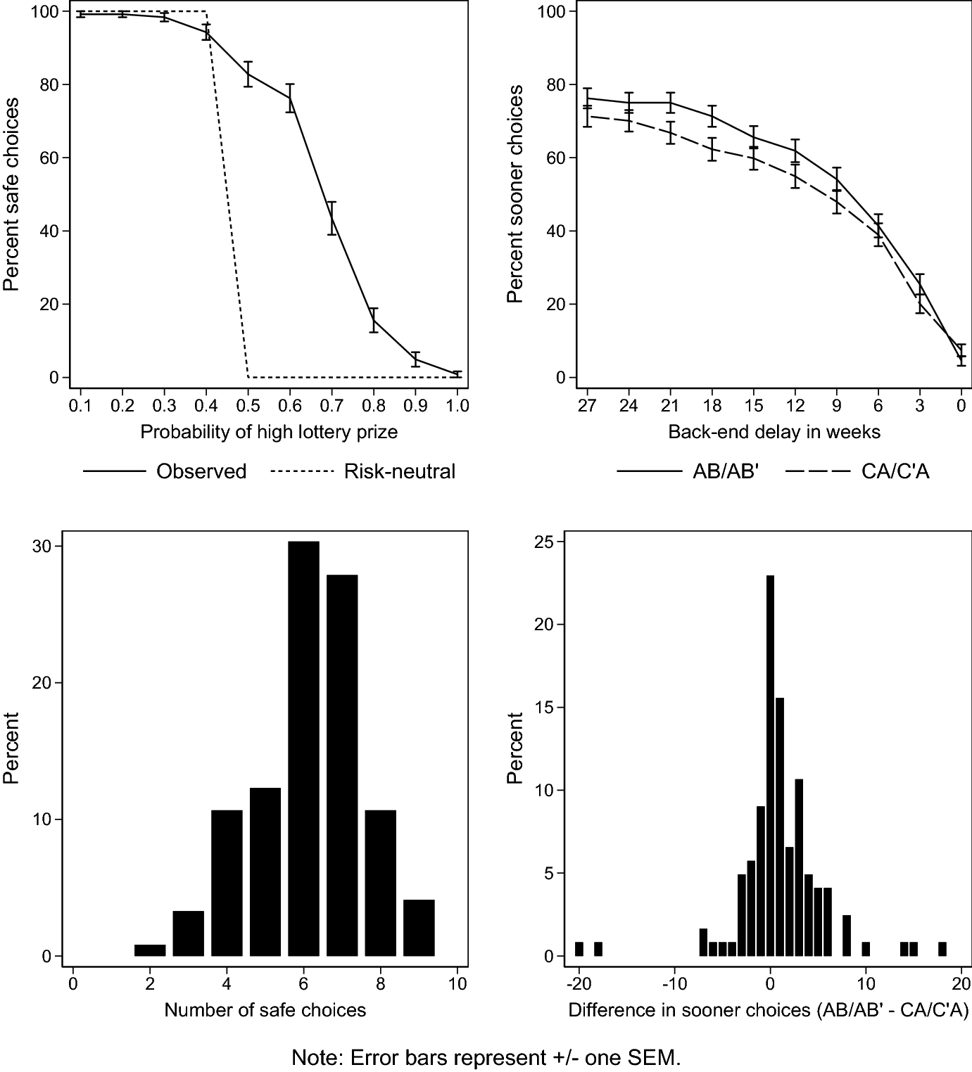
Fig. 4 Choice behavior in risk and time preference tasks

Turning to behavior in time preference tasks, the upper right panel reports the percentage of smaller-sooner choices as a function of the back-end delay, separately for the pooled AB/AB’ and CA/C’A choice lists. Appendix B.1 reports separate figures for each list. The proportion of sooner choices declines smoothly as the back-end delay falls and the interest rate increases, suggesting that subjects understood the underlying trade-off entailed in waiting a longer or shorter time for a given-sized increase in undiscounted payoffs.

Under linear utility subjects are predicted to make the same choices in all lists, while departures from linearity are expressed as differences across lists. In particular, a subject with concave utility prefers to smooth payoffs over time, and thus makes more sooner choices in AB/AB’ choice lists (in which the smaller-sooner option is more temporally balanced) than in CA/C’A lists (in which the larger-later option is more balanced). The upper right panel of Fig. 4 confirms a small, but clearly discernible shift in the direction predicted by concave utility. At every back-end delay except zero (where the sooner option is dominated), subjects make more sooner choices in AB/AB’ than in CA/C’A. To illustrate the magnitude of these differences, the error bars represent ± one standard error of the mean for a binomial proportion.

The lower right panel of Fig. 4 reports a histogram of the difference in the number of sooner choices made by each subject between the AB/AB’ and CA/C’A choice lists. The mode of this distribution is at zero, corresponding to linear utility, but there is greater mass to the right indicating a tendency toward concavity. The median subject makes a total of 13 sooner choices in the combined AB/AB’ choice lists, compared to 11.5 in the CA/C’A lists. This difference is highly significant, with $p=0.0013$ in a sign test, or $p=0.0006$ in a Wilcoxon signed-ranks test.Footnote ²² This evidence of a systematic tendency to prefer the more balanced payoff vector A, consistent with a preference to smooth payoffs over time, does not rely on any assumptions on the functional form of utility.Footnote ²³

Figure 4 establishes that, in both risk and time preference, there is clear evidence of the choice patterns implied by concave utility. The finding for risk replicates other studies that use the HL design, while the finding for time is a novel result of transposing that design into the domain of time preference. Moreover, while both effects are highly significant, it is clear that the magnitude is smaller in choice over time. This suggests that while instantaneous utility for time is indeed concave, it may be less concave than Bernoulli utility for risk. To formalize this observation, I next estimate structural preference models for a representative agent, building upon well-established procedures documented by Harrison and Rutström (Reference Harrison, Rutström, Cox and Harrison2008) for risk and Andersen et al. (Reference Andersen, Harrison, Lau and Rutström2008, Reference Andersen, Harrison, Lau and Rutström2014) for time.

3.2 Utility curvature under risk

For risk preference, I assume a constant relative risk aversion (CRRA) functional form for Bernoulli utility:

(5) $\begin{array}{c}u\left(x\right)=\frac{x^{1-\alpha }}{1-\alpha }\end{array}$

such that $\alpha =0$ corresponds to linear utility, while $\alpha >0$ implies concave utility. I begin with expected utility, but the exposition treats this as the special case of rank-dependent utility with $w\left(p\right)=p$ . Given some candidate value of $\alpha$ (and probability weighting parameters), the rank-dependent utility of each lottery is evaluated. Then, adopting a “contextual” error specification (Wilcox Reference Wilcox2011), the probability that Option B is chosen is modeled as:

(6) $\begin{array}{c}Pr\left(B\right)=\Lambda \left(\left(\left(R,D,U_B,-,R,D,U_A\right),/,\nu \right),/,\mu \right)\end{array}$

where $\Lambda \left(·\right)$ is the cumulative logistic distribution function, $\nu$ is the difference between the maximum and minimum utilities over all prizes in the choice set,Footnote ²⁴ and $\mu$ is a structural “noise” parameter for the risk preference choices. As $\mu$ goes to zero, the lottery with the larger RDU is chosen deterministically, while as $\mu$ goes to infinity, the choice probability goes to one-half such that choices are essentially random. The data consists of 1220 observations, being ten binary choices in the risk preference task for each of 122 subjects. The parameters are estimated to maximize the likelihood of the observed choices using Stata 16, with robust standard errors clustered at the level of individual subjects.

Model (1) in Table 1 reports estimates under expected utility. The point estimate of $\alpha$ is 0.547, with a standard error of 0.036. This implies substantial concavity of Bernoulli utility, and sits comfortably within the range of previously-reported estimates using similar experimental designs and estimation procedures.Footnote ²⁵

Table 1 Representative agent estimates of utility curvature and discount rates

	(1)	(2)	(3)	(4)	(5)	(6)	(7)	(8)
	EU	RDU	Linear	Linear-CB	DU	Joint-EU	Joint-RDU	DIU
CRRA utility curvature ( $\alpha$ , $\theta$ , $\Theta$ )	0.547	0.206			0.018	0.456	0.421	0.226
	(0.036)	(0.095)			(0.006)	(0.012)	(0.020)	(0.060)
Probability weighting ( $\eta$ , $\gamma$ )		0.788					0.789
		(0.280)					(0.052)
Annual discount rate ( $\rho$ )			0.639	0.622	0.626	0.065	0.107	0.504
			(0.077)	(0.075)	(0.074)	(0.017)	(0.025)	(0.063)
Decision “noise” for risk ( $\mu$ )	0.082	0.088				0.083	0.073
	(0.009)	(0.009)				(0.008)	(0.009)
Decision “noise” for time ( $\sigma$ )			0.028	0.034	0.028	0.006	0.009	0.027
			(0.002)	(0.003)	(0.002)	(0.002)	(0.002)	(0.002)
AIC	689.875	685.734	8807.895	1412.456	8790.165	2082.889	2061.119	8785.710
BIC	700.089	701.054	8821.692	1422.670	8810.860	2106.088	2090.117	8806.405
LL	– 342.938	– 339.867	– 4401.948	– 704.228	– 4392.083	– 1037.445	– 1025.559	– 4389.855
Probability weighting function		Gul					Prelec-I
Risk preference data	Yes	Yes				Yes	Yes
Time preference data			Yes	CB only	Yes	CB only	CB only	Yes
N	1220	1220	7320	1220	7320	2440	2440	7320

Cluster robust standard errors in parentheses

As discussed in Sect. 2.1, risk aversion in HL-style tasks may be driven by curvature of the utility function, and/or by non-linear probability weighting. Therefore, just as assuming linear utility may cause estimates of the discount rate to be biased in choice over time, assuming linear probability weighting may cause estimates of the utility function to be biased in choice under risk. Indeed, Drichoutis and Lusk (Reference Drichoutis and Lusk2016) claim that risk aversion in HL tasks may be solely a product of probability weighting as opposed to utility curvature: in their estimates of a rank-dependent model they find significant non-linear probability weighting, while the CRRA coefficient does not differ significantly from zero. While this finding is arguably at odds with other existing literature,Footnote ²⁶ it highlights the importance of allowing for probability weighting when comparing the curvature of utility elicited under risk and over time.

To examine the robustness of concave Bernoulli utility to the possibility of non-linear probability weighting, I estimate rank-dependent models for each parametric form of the probability weighting function in Section 3.6 of the survey by Fehr-Duda and Epper (Reference Fehr-Duda and Epper2012). The Bayesian information criterion (BIC) in fact selects the expected utility specification of model (1) in Table 1. The Akaike information criterion (AIC), which penalizes model complexity less severely than the BIC, selects a model with a single-parameter weighting function from the theory of disappointment aversion of Gul (Reference Gul1991): $w\left(p\right)=p/\left(1,+,\left(1,-,p\right),\eta \right)$ . The resulting estimates are set out as model (2) in Table 1. This weighting function simplifies to linearity at $\eta =0$ , a restriction that is clearly rejected with $p=0.005$ . The implied weighting function is convex, and is depicted by the dashed line in Fig. 5. For the purpose of this paper, the effect on the estimate of utility curvature is of greatest interest. This estimate is now smaller (and less precisely estimated) than under expected utility. However, it will transpire that it is still considerably greater than the curvature of instantaneous utility estimated from choices over time.

Fig. 5 Estimated probability weighting functions

3.3 Utility curvature and discounting over time

I next set out how the data from the six time preference choice lists can be used to estimate both the curvature of instantaneous utility and the discount rate, adopting similar procedures to Sect. 3.2 and Andersen et al. (Reference Andersen, Harrison, Lau and Rutström2008, Reference Andersen, Harrison, Lau and Rutström2014). I assume a CRRA form for the instantaneous utility function:

(7) $\begin{array}{c}v\left(x\right)=\frac{x^{1-\theta }}{1-\theta }\end{array}$

and an exponential form for the discount function:

(8) $\begin{array}{c}D\left(t\right)=\frac{1}{{\left(1,+,\rho \right)}^{\frac{t}{52}}}\end{array}$

where $\theta$ captures the curvature of instantaneous utility and $\rho$ is the annual discount rate. Given candidate values of $\theta$ and $\rho$ , the discounted utility of each alternative is evaluated and the probability that the alternative presented as Option B is chosen is modeled as:

(9) $\begin{array}{c}Pr\left(B\right)=\Lambda \left(\left(\left(D,U_B,-,D,U_A\right),/,\lambda \right),/,\sigma \right)\end{array}$

where $\lambda$ is a contextual normalization term,Footnote ²⁷ and $\sigma$ is a noise parameter for the time preference choices.

It is worth emphasizing that this framework is essentially the same as that of Andersen et al. (Reference Andersen, Harrison, Lau and Rutström2008, Reference Andersen, Harrison, Lau and Rutström2014), except that information on utility curvature is obtained directly from choices over time instead of a separate risk preference task, so it is not necessary to equate Bernoulli utility for risk with instantaneous utility for time. The data consists of 7320 observations, being ten binary choices in each of six time preference choice lists for each of 122 subjects. The parameters $\theta$ , $\rho$ , and $\sigma$ are estimated by maximum likelihood in Stata 16, with robust standard errors clustered at the level of individual subjects.

Before turning to the full results, model (3) in Table 1 reports a linear utility specification, with $\theta$ constrained to zero, giving an estimated annual discount rate of 63.9%. While this is higher than prevailing market interest rates, it is not extreme by the standards of the literature.Footnote ²⁸ Model (4) reports a linear utility specification using only the data of the CB choice list in which the smaller-sooner option pays $\left(\$,33,,,\$,2\right)$ while larger-later pays $\left(\$,1,,,\$,38\right)$ . This is included for comparability with more conventional designs that offer all-sooner or all-later payments, as well as the subsequent replication of joint estimation invoking utility from the risk preference task in Sect. 3.4. The resulting estimate of the discount rate is very close to that of model (3).

Model (5) reports the main discounted utility estimates, allowing non-linear instantaneous utility revealed through data on choices over time. In this model, the point estimate of $\theta$ is 0.018 with a standard error of 0.006, indicating significantly concave utility. This is consistent with the model-free analysis in Sect. 3.1. However, the estimate of $\theta$ is an order of magnitude smaller than estimates of $\alpha$ from risk preference data in models (1) and (2). Because the estimated curvature of instantaneous utility is modest, the effect of correcting for this concavity upon the discount rate is mild: the estimate of $\rho$ falls from 63.9% in model (3) to 62.6% in model (5). Both the AIC and BIC select the non-linear utility specification of model (5) over the more parsimonious linear utility specification in model (3).

3.4 Joint estimation

The modest effect of correcting for the curvature of instantaneous utility may be contrasted with that of a joint estimation procedure that combines risk and time preference data and imposes a single utility function upon both. To illustrate, I pool the data of the risk task with that of the CB choice list, which is comparable to conventional time preference data in that the payoffs are essentially at the all-sooner or all-later corners. The probability of making a risky lottery choice is modeled by Eq. 6 while that of making a larger-later choice is modeled by Eq. 9. The noise terms $\mu$ and $\sigma$ are allowed to differ across risk and time preference tasks, but the utility function is constrained to be the same for both, such that $\alpha =\theta$ . The data consists of 2440 observations, being ten risk and ten time preference choices for each of 122 subjects, and the parameters are estimated to maximize the joint likelihood of both sets of choices.

Model (6) in Table 1 reports joint estimates assuming expected utility for risk. The estimate of utility curvature is 0.456 with a standard error of 0.012, reflecting the influence of risk aversion in the lottery choices, while the estimated annual discount rate falls to 6.5%. This compares to an estimate of 62.2% in model (4), which uses the same CB time preference data but assumes linear utility.

To allow for non-linear probability weighting in the risk preference data, I again re-estimate the joint model assuming rank-dependent utility for each parametric weighting function in Fehr-Duda and Epper (Reference Fehr-Duda and Epper2012). The effect upon utility and discounting is very similar across all specifications: the estimate of utility curvature falls to between 0.419 and 0.427 while the estimated discount rate increases slightly to between 10.0 and 10.9%. Both the AIC and BIC select a specification with a single-parameter weighting function from Prelec (Reference Prelec1998): $w\left(p\right)=exp\left(-,{\left(-,ln,\left(p\right)\right)}^{\gamma }\right)$ , and the resulting estimates are reported as model (7) in Table 1. This weighting function simplifies to linearity at $\gamma =1$ , a restriction that is rejected with $p<0.0001$ in a Wald test. The implied weighting function is inverse-S shaped, and is depicted by the solid line in Fig. 5.

For the purpose of this paper, the key conclusions are twofold. First, even allowing for probability weighting, joint estimates of utility curvature which impose the restriction that $\alpha =\theta$ are considerably larger than the discounted utility estimate in model (5) which imposes no such restriction. Second, relative to the linear utility benchmark of model (4), the effect upon the discount rate of correcting for this amount of curvature is dramatic. The discount rates in models (6) and (7) are substantially smaller than the lowest interest rate offered in the experiment, suggesting that joint estimation may have yielded an over-correction.

3.5 Discounted incremental utility

In Sects. 3.3 and 3.4, and models (3) through (7) in Table 1, I explored the effect of alternative assumptions about the nature of instantaneous utility—whether it is taken to be linear as in models (3) and (4), revealed through responses to varying opportunities for intertemporal substitution as in model (5), or equated with Bernoulli utility for risk as in models (6) and (7). It was assumed throughout that the underlying framework to evaluate streams of payoffs over time is given by the discounted utility model in Eq. 3.

Blavatskyy (Reference Blavatskyy2016) has argued that discounted utility may give rise to violations of intertemporal monotonicity when utility is not linear. In particular, it is possible for discounted utility to increase when a payoff is split into two parts, one of which is slightly delayed. That is, if $v\left(x\right)$ is sufficiently concave while $D\left(t,+,k\right)$ is close to $D\left(t\right)$ it is possible to have:

$\begin{array}{c}D\left(t\right)·v\left(x\right)<D\left(t\right)·v\left(x,/,2\right)+D\left(t,+,k\right)·v\left(x,/,2\right)\end{array}$

This implies that there may be a benefit to delay without any compensating increase in the magnitude of the payoff. The issue occurs when the impact of diminishing marginal utility as a payoff is divided in two outweighs the impact of discounting as a portion of it is delayed. This may occur in any model that has the discounted utility structure of Eq. 3, and is not specific to any functional form of the discount function $D\left(t\right)$ such as exponential discounting. Assuming discounted utility, it can be avoided only if utility is linear. It thus represents a theoretical argument for why discounted utility may be incompatible with substantial non-linearity of instantaneous utility, as found empirically in model (5) of Table 1.

The argument of Blavatskyy (Reference Blavatskyy2016) is analogous to how simple probability weighting may violate first-order stochastic dominance in the original prospect theory of Kahneman and Tversky (Reference Kahneman and Tversky1979). In that setting, the solution proposed by Quiggin (Reference Quiggin1982) is to construct decision weights from a transformation of the cumulative probabilities instead of directly transforming the probabilities themselves. In the context of time, the solution proposed by Blavatskyy (Reference Blavatskyy2016) is to apply a utility transformation to the cumulative payoffs instead of directly to the payoffs themselves. This gives rise to the model of discounted incremental utility (Blavatskyy Reference Blavatskyy2016, equation 3) which replaces discounted utility by:

(10) $\begin{array}{c}DIU\left(x_t,,,t,;,,x_{t+k},,,t,+,k\right)=D\left(t\right)·V\left(x_t\right)+D\left(t,+,k\right)·\left(V,\left(x_t,+,x_{t+k}\right),-,V,\left(x_t\right)\right)\end{array}$

This states that future payoffs are evaluated by the discounted value of their incremental contribution to the utility of the cumulated payoffs, $V\left(·\right)$ .

Estimation of the discounted incremental model requires data on choices over non-degenerate streams, such as that reported in this paper,Footnote ²⁹ as opposed to conventional choices over all-sooner versus all-later payoffs which never cumulate. If the cumulative utility function is linear then Eq. 10, like Eq. 3, simplifies to discounted linear utility, in which case a subject is again predicted to have the same switch point in all six choice lists. However if the cumulative utility function is concave, I show in Appendix A.3 that discounted incremental utility again predicts a later switch point in AB/AB’ than in CA/C’A choice lists.

To estimate the model I again assume a CRRA form, this time for the utility of cumulated payoffs, X:

(11) $\begin{array}{c}V\left(X\right)=\frac{X^{1-\Theta }}{1-\Theta }\end{array}$

and the exponential discount function of Eq. 8, and define choice probabilities analogously to Eq. 9 except replacing DU by DIU. The model is estimated using the same set of 7320 observations from six time preference choice lists as used in models (3) and (5) of Table 1.

Estimates of the discounted incremental specification are reported as model (8) in Table 1. The curvature of cumulative utility is significantly concave, with a CRRA coefficient of 0.226 and standard error of 0.060. This is substantially larger than the estimated curvature of instantaneous utility in the discounted utility specification of model (5). Allowing for this amount of curvature reduces the estimate of the annual discount rate from 63.9% under linear utility in model (3) to 50.4% in model (8). The discounted incremental specification has the same number of parameters as the discounted utility model, and a superior log-likelihood. As a result, both the AIC and BIC select this model over both the discounted utility and linear models.

3.6 Robustness checks

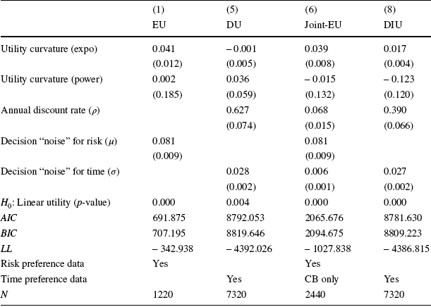
In this section, I report several robustness checks of the key representative agent estimates to alternative structural assumptions. Table 2 reports expected utility, discounted utility, joint, and discounted incremental estimates assuming a constant absolute risk aversion form for utility: $u\left(x\right)=\left(1,-,exp,\left(-,a,x\right)\right)/a$ . Table 3 reports corresponding estimates assuming expo-power utility (Saha Reference Saha1993; Holt and Laury Reference Holt and Laury2002): $u\left(x\right)=\left(1,-,exp,\left(-,a,x^{1-r}\right)\right)/a$ . These analyses replicate all key implications of Table 1: instantaneous utility in model (5) is significantly concaveFootnote ³⁰ though substantially less so than Bernoulli utility in model (1); the discount rate in model (5) is only marginally smaller than that assuming linear utility (c.f. Table 1, model (3)), whereas the one obtained from joint estimation in model (6) is substantially lower; and the effects of discounted incremental utility in model (8) are similar to those in Table 1.

Table 2 Representative agent estimates under CARA utility

	(1)	(5)	(6)	(8)
	EU	DU	Joint-EU	DIU
CARA utility curvature	0.041	0.001	0.040	0.018
	(0.003)	(0.000)	(0.002)	(0.005)
Annual discount rate ( $\rho$ )		0.624	0.068	0.424
		(0.073)	(0.016)	(0.065)
Decision “noise” for risk ( $\mu$ )	0.081		0.081
	(0.009)		(0.009)
Decision “noise” for time ( $\sigma$ )		0.028	0.006	0.027
		(0.002)	(0.001)	(0.002)
AIC	689.875	8790.505	2063.699	8780.517
BIC	700.089	8811.200	2086.898	8801.212
LL	– 342.938	– 4392.252	– 1027.849	– 4387.259
Risk preference data	Yes		Yes
Time preference data		Yes	CB only	Yes
N	1220	7320	2440	7320

Clustered standard errors in parentheses. Column numbers indicate corresponding models in Table 1

Table 3 Representative agent estimates under expo-power utility

	(1)	(5)	(6)	(8)
	EU	DU	Joint-EU	DIU
Utility curvature (expo)	0.041	– 0.001	0.039	0.017
	(0.012)	(0.005)	(0.008)	(0.004)
Utility curvature (power)	0.002	0.036	– 0.015	– 0.123
	(0.185)	(0.059)	(0.132)	(0.120)
Annual discount rate ( $\rho$ )		0.627	0.068	0.390
		(0.074)	(0.015)	(0.066)
Decision “noise” for risk ( $\mu$ )	0.081		0.081
	(0.009)		(0.009)
Decision “noise” for time ( $\sigma$ )		0.028	0.006	0.027
		(0.002)	(0.001)	(0.002)
$H_0$ : Linear utility (p-value)	0.000	0.004	0.000	0.000
AIC	691.875	8792.053	2065.676	8781.630
BIC	707.195	8819.646	2094.675	8809.223
LL	– 342.938	– 4392.026	– 1027.838	– 4386.815
Risk preference data	Yes		Yes
Time preference data		Yes	CB only	Yes
N	1220	7320	2440	7320

Clustered standard errors in parentheses. Column numbers indicate corresponding models in Table 1

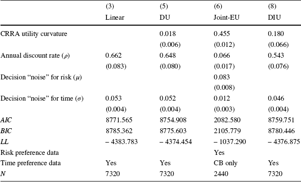
Table 4 reports linear, discounted utility, joint, and discounted incremental estimates for CRRA utility using an alternative contextual normalization that replaces the expression in footnote 27 with $\lambda =v\left(x_{\max }\right)-v\left(x_{\min }\right)$ (see Blavatskyy and Maafi Reference Blavatskyy and Maafi2018, p. 278). That is, instead of normalizing by the difference in discounted utilities between the best and worst payoff streams, these estimates normalize by the difference in instantaneous utilities between the best and worst payoffs, which does not depend upon the discount function.Footnote ³¹ Again, all key implications of Table 1 are maintained.

Table 4 Representative agent estimates under alternative contextual normalization

	(3)	(5)	(6)	(8)
	Linear	DU	Joint-EU	DIU
CRRA utility curvature		0.018	0.455	0.180
		(0.006)	(0.012)	(0.066)
Annual discount rate ( $\rho$ )	0.662	0.648	0.066	0.543
	(0.083)	(0.080)	(0.017)	(0.076)
Decision “noise” for risk ( $\mu$ )			0.083
			(0.008)
Decision “noise” for time ( $\sigma$ )	0.053	0.052	0.012	0.046
	(0.004)	(0.004)	(0.003)	(0.004)
AIC	8771.565	8754.908	2082.580	8759.751
BIC	8785.362	8775.603	2105.779	8780.446
LL	– 4383.783	– 4374.454	– 1037.290	– 4376.875
Risk preference data			Yes
Time preference data	Yes	Yes	CB only	Yes
N	7320	7320	2440	7320

Clustered standard errors in parentheses. Column numbers indicate corresponding models in Table 1

3.7 Individual estimation and prediction

In this section, I extend the analysis to estimation at an individual level, and examine the performance of individual estimates in predicting subjects’ choices in the risk and time preference decisions respectively.

In the full sample of 122 subjects there are fifteen who choose larger-later in all 60 time preference decisions, and four who choose smaller-sooner in all 54 decisions where it is not dominated. I thus focus on the remaining 103 subjects in individual estimation. Since there is only a single risk preference choice list, it is not possible to estimate probability weighting parameters at an individual level. I thus report individual estimates for five models: the expected utility specification in model (1) of Table 1, the linear utility specification in model (3), the discounted utility specification in model (5), the joint estimation specification in model (6), and the discounted incremental specification in model (8). Individual estimation was performed in Matlab R2018b, after first replicating the corresponding representative agent estimates from Table 1.

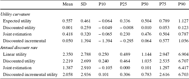
Table 5 reports summary statistics for four individual measures of CRRA utility curvature (not estimated under linear utility) and four individual estimates of the annual discount rate (not estimated under expected utility). Histograms for each set of estimates are reported in Appendix B.2. For utility curvature, the mean and median estimates under expected utility, discounted utility and joint estimation are very similar to the corresponding representative agent estimates. However for discounted incremental utility, the mean and median curvature are closer to linearity than the aggregate estimate, and the variance is considerable. For discounting, the mean and median estimates are consistently larger than the corresponding estimates in Table 1, in part reflecting the fact that the individual estimation sample excludes the fifteen most patient subjects.Footnote ³²

Table 5 Summary statistics of individual utility curvature and discount rate estimates

	Mean	SD	P10	P25	P50	P75	P90
Utility curvature
Expected utility	0.557	0.461	– 0.064	0.336	0.504	0.789	1.127
Discounted utility	0.001	0.259	– 0.049	– 0.008	0.010	0.053	0.123
Joint estimation	0.418	0.320	– 0.065	0.230	0.476	0.504	0.787
Discounted incremental	0.050	1.394	– 1.394	– 0.295	0.064	0.577	1.056
Annual discount rate
Linear utility	2.350	2.788	0.250	0.489	1.144	2.947	6.904
Discounted utility	2.219	2.699	0.240	0.464	1.035	2.535	6.707
Joint estimation	1.387	2.910	– 0.105	0.000	0.101	1.297	6.417
Discounted incremental utility	2.058	2.936	0.101	0.306	0.783	2.616	6.703

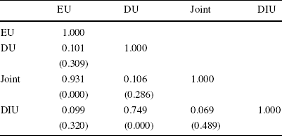
Table 6 reports the Spearman rank correlation matrix for the four individual measures of utility curvature. This strongly supports the conjecture that risk and time preferences reflect two distinct notions of utility. On one hand, the expected utility and joint estimates, which infer curvature from choices under risk, are highly significantly correlated. On the other hand, the discounted utility and discounted incremental estimates, which infer curvature from choices over time, are also highly significantly correlated. However the remaining four coefficients, which compare one measure elicited under risk to another measure elicited over time, are consistently small (Spearman rho less than 0.11) and far from statistically significant.

Table 6 Spearman rank correlation matrix of individual utility curvature estimates

	EU	DU	Joint	DIU
EU	1.000
DU	0.101	1.000
	(0.309)
Joint	0.931	0.106	1.000
	(0.000)	(0.286)
DIU	0.099	0.749	0.069	1.000
	(0.320)	(0.000)	(0.489)

p-values in parentheses

Figure 6 depicts a scatter plot of the individual estimates of $\alpha$ under expected utility and $\theta$ under discounted utility, these being the standard normative benchmarks for risk and time preference respectively.Footnote ³³ According to the model of discounted expected utility, these measures are interchangeable and so all points should lie on a 45-degree diagonal. Instead, not only do the two sets of estimates differ considerably in magnitude, they are also essentially uncorrelated.Footnote ³⁴

Fig. 6 Scatter plot of individual estimates of $\alpha$ and $\theta$

To further examine the implications of alternative assumptions regarding the nature of utility, I use each set of estimates to generate predicted choices for each subject in each of the ten risk and 60 time preference decisions, and compare these predictions to their actual choices.Footnote ³⁵

For risk preference, simply assuming linear utility (i.e., that every subject switches from safe to risky after four rows) suffices to correctly predict 76.7% of the data. Relative to this benchmark, individual curvature estimates from the discounted utility model correctly predict 76.8% of risk preference choices, while those of the discounted incremental model correctly predict 74.6%. Treating individual subjects as independent observations, the proportion of their choices correctly predicted by either model does not differ significantly from the proportion correctly predicted by linear utility, in either a sign test or a signed-ranks test. By contrast, individual expected utility estimates correctly predict 98.5% of choices, and joint estimates 95.0%, both improving significantly upon linear utility with $p<0.0001$ in both a sign test and a signed-ranks test.

For time preference, individual discount rates assuming linear utility correctly predict 86.6% of the data. This increases to 89.4% allowing non-linear utility in a discounted utility model, or 87.3% in a discounted incremental model. Again treating individual subjects as independent observations, both sets of estimates improve significantly upon linear utility.Footnote ³⁶ By contrast, individual joint estimates correctly predict only 68.4% of the data. Recall that joint estimation uses only the CB choice list for time. Individual linear utility estimates using only CB data (corresponding to model (4) in Table 1) correctly predict 84.1% of the data. The individual joint estimates predict significantly worse than this linear-CB benchmark, with $p<0.0001$ in both a sign test and a signed-ranks test.

Figure 7 examines prediction performance of individual estimates in greater detail. The top panel relates to the risk preference task, while the lower two panels pool the AB/AB’ and CA/C’A choice lists for time, respectively. In each panel, the solid line depicts observed safe or sooner choices at each row.Footnote ³⁷ The shorter-dashed line depicts predictions of the joint estimation model (which infers utility curvature from choice under risk), while the longer-dashed line depicts predictions of the discounted utility model (which infers curvature from choice over time). The comparison between these predictions thus illustrates the effect of assuming equivalence between Bernoulli and instantaneous utility versus allowing for them to be separated. The figure illustrates how both sets of estimates make poor out-of-sample predictions, because they reflect quantitatively different degrees of concavity. Since instantaneous utility for time is near-linear, it wrongly predicts near risk-neutral behavior in choice under risk. But conversely, since Bernoulli utility for risk is more concave, it greatly exaggerates the preference for the temporally-balanced payoff vector A, both when it is smaller-sooner as in AB/AB’, and when it is larger-later as in CA/C’A.

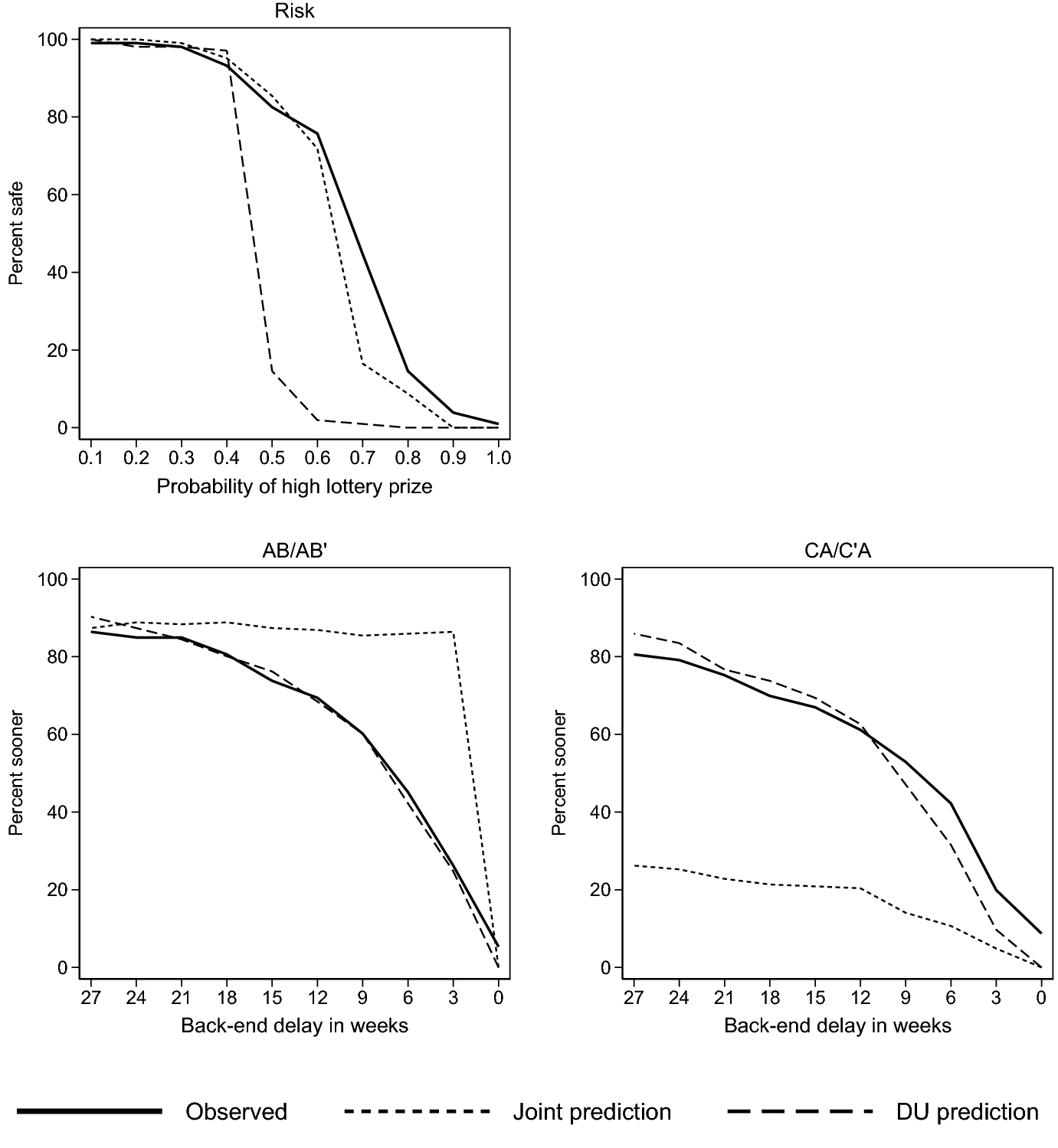
Fig. 7 Prediction performance of individual estimates